Chapter 10. Neural Networks
“You can’t process me with a normal brain.” — Charlie Sheen
We’re at the end of our story. This is the last official chapter of this book (though I envision additional supplemental material for the website and perhaps new chapters in the future). We began with inanimate objects living in a world of forces and gave those objects desires, autonomy, and the ability to take action according to a system of rules. Next, we allowed those objects to live in a population and evolve over time. Now we ask: What is each object’s decision-making process? How can it adjust its choices by learning over time? Can a computational entity process its environment and generate a decision?
The human brain can be described as a biological neural network—an interconnected web of neurons transmitting elaborate patterns of electrical signals. Dendrites receive input signals and, based on those inputs, fire an output signal via an axon. Or something like that. How the human brain actually works is an elaborate and complex mystery, one that we certainly are not going to attempt to tackle in rigorous detail in this chapter.
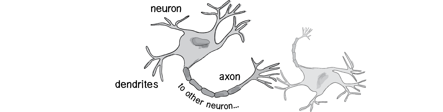
Figure 10.1
The good news is that developing engaging animated systems with code does not require scientific rigor or accuracy, as we’ve learned throughout this book. We can simply be inspired by the idea of brain function.
In this chapter, we’ll begin with a conceptual overview of the properties and features of neural networks and build the simplest possible example of one (a network that consists of a single neuron). Afterwards, we’ll examine strategies for creating a “Brain” object that can be inserted into our Vehicle class and used to determine steering. Finally, we’ll also look at techniques for visualizing and animating a network of neurons.
10.1 Artificial Neural Networks: Introduction and Application
Computer scientists have long been inspired by the human brain. In 1943, Warren S. McCulloch, a neuroscientist, and Walter Pitts, a logician, developed the first conceptual model of an artificial neural network. In their paper, "A logical calculus of the ideas imminent in nervous activity,” they describe the concept of a neuron, a single cell living in a network of cells that receives inputs, processes those inputs, and generates an output.
Their work, and the work of many scientists and researchers that followed, was not meant to accurately describe how the biological brain works. Rather, an artificial neural network (which we will now simply refer to as a “neural network”) was designed as a computational model based on the brain to solve certain kinds of problems.
It’s probably pretty obvious to you that there are problems that are incredibly simple for a computer to solve, but difficult for you. Take the square root of 964,324, for example. A quick line of code produces the value 982, a number Processing computed in less than a millisecond. There are, on the other hand, problems that are incredibly simple for you or me to solve, but not so easy for a computer. Show any toddler a picture of a kitten or puppy and they’ll be able to tell you very quickly which one is which. Say hello and shake my hand one morning and you should be able to pick me out of a crowd of people the next day. But need a machine to perform one of these tasks? Scientists have already spent entire careers researching and implementing complex solutions.
The most common application of neural networks in computing today is to perform one of these “easy-for-a-human, difficult-for-a-machine” tasks, often referred to as pattern recognition. Applications range from optical character recognition (turning printed or handwritten scans into digital text) to facial recognition. We don’t have the time or need to use some of these more elaborate artificial intelligence algorithms here, but if you are interested in researching neural networks, I’d recommend the books Artificial Intelligence: A Modern Approach by Stuart J. Russell and Peter Norvig and AI for Game Developers by David M. Bourg and Glenn Seemann.
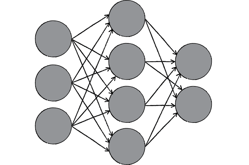
Figure 10.2
A neural network is a “connectionist” computational system. The computational systems we write are procedural; a program starts at the first line of code, executes it, and goes on to the next, following instructions in a linear fashion. A true neural network does not follow a linear path. Rather, information is processed collectively, in parallel throughout a network of nodes (the nodes, in this case, being neurons).
Here we have yet another example of a complex system, much like the ones we examined in Chapters 6, 7, and 8. The individual elements of the network, the neurons, are simple. They read an input, process it, and generate an output. A network of many neurons, however, can exhibit incredibly rich and intelligent behaviors.
One of the key elements of a neural network is its ability to learn. A neural network is not just a complex system, but a complex adaptive system, meaning it can change its internal structure based on the information flowing through it. Typically, this is achieved through the adjusting of weights. In the diagram above, each line represents a connection between two neurons and indicates the pathway for the flow of information. Each connection has a weight, a number that controls the signal between the two neurons. If the network generates a “good” output (which we’ll define later), there is no need to adjust the weights. However, if the network generates a “poor” output—an error, so to speak—then the system adapts, altering the weights in order to improve subsequent results.
There are several strategies for learning, and we’ll examine two of them in this chapter.
Supervised Learning —Essentially, a strategy that involves a teacher that is smarter than the network itself. For example, let’s take the facial recognition example. The teacher shows the network a bunch of faces, and the teacher already knows the name associated with each face. The network makes its guesses, then the teacher provides the network with the answers. The network can then compare its answers to the known “correct” ones and make adjustments according to its errors. Our first neural network in the next section will follow this model.
Unsupervised Learning —Required when there isn’t an example data set with known answers. Imagine searching for a hidden pattern in a data set. An application of this is clustering, i.e. dividing a set of elements into groups according to some unknown pattern. We won’t be looking at any examples of unsupervised learning in this chapter, as this strategy is less relevant for our examples.
Reinforcement Learning —A strategy built on observation. Think of a little mouse running through a maze. If it turns left, it gets a piece of cheese; if it turns right, it receives a little shock. (Don’t worry, this is just a pretend mouse.) Presumably, the mouse will learn over time to turn left. Its neural network makes a decision with an outcome (turn left or right) and observes its environment (yum or ouch). If the observation is negative, the network can adjust its weights in order to make a different decision the next time. Reinforcement learning is common in robotics. At time t, the robot performs a task and observes the results. Did it crash into a wall or fall off a table? Or is it unharmed? We’ll look at reinforcement learning in the context of our simulated steering vehicles.
This ability of a neural network to learn, to make adjustments to its structure over time, is what makes it so useful in the field of artificial intelligence. Here are some standard uses of neural networks in software today.
Pattern Recognition —We’ve mentioned this several times already and it’s probably the most common application. Examples are facial recognition, optical character recognition, etc.
Time Series Prediction —Neural networks can be used to make predictions. Will the stock rise or fall tomorrow? Will it rain or be sunny?
Signal Processing —Cochlear implants and hearing aids need to filter out unnecessary noise and amplify the important sounds. Neural networks can be trained to process an audio signal and filter it appropriately.
Control —You may have read about recent research advances in self-driving cars. Neural networks are often used to manage steering decisions of physical vehicles (or simulated ones).
Soft Sensors —A soft sensor refers to the process of analyzing a collection of many measurements. A thermometer can tell you the temperature of the air, but what if you also knew the humidity, barometric pressure, dewpoint, air quality, air density, etc.? Neural networks can be employed to process the input data from many individual sensors and evaluate them as a whole.
Anomaly Detection —Because neural networks are so good at recognizing patterns, they can also be trained to generate an output when something occurs that doesn’t fit the pattern. Think of a neural network monitoring your daily routine over a long period of time. After learning the patterns of your behavior, it could alert you when something is amiss.
This is by no means a comprehensive list of applications of neural networks. But hopefully it gives you an overall sense of the features and possibilities. The thing is, neural networks are complicated and difficult. They involve all sorts of fancy mathematics. While this is all fascinating (and incredibly important to scientific research), a lot of the techniques are not very practical in the world of building interactive, animated Processing sketches. Not to mention that in order to cover all this material, we would need another book—or more likely, a series of books.
So instead, we’ll begin our last hurrah in the nature of code with the simplest of all neural networks, in an effort to understand how the overall concepts are applied in code. Then we’ll look at some Processing sketches that generate visual results inspired by these concepts.
10.2 The Perceptron
Invented in 1957 by Frank Rosenblatt at the Cornell Aeronautical Laboratory, a perceptron is the simplest neural network possible: a computational model of a single neuron. A perceptron consists of one or more inputs, a processor, and a single output.
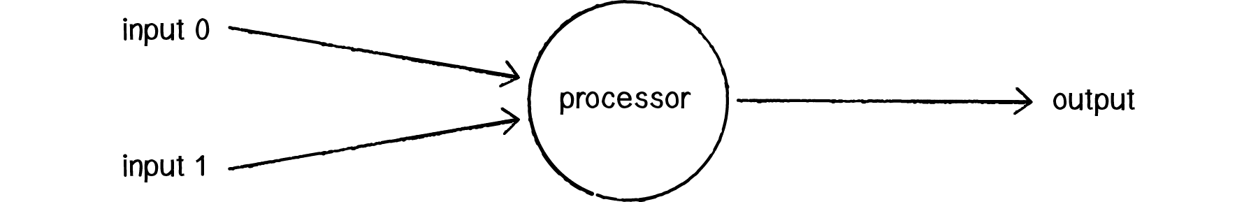
Figure 10.3: The perceptron
A perceptron follows the “feed-forward” model, meaning inputs are sent into the neuron, are processed, and result in an output. In the diagram above, this means the network (one neuron) reads from left to right: inputs come in, output goes out.
Let’s follow each of these steps in more detail.
Step 1: Receive inputs.
Say we have a perceptron with two inputs—let’s call them x1 and x2.
Input 0: x1 = 12
Input 1: x2 = 4
Step 2: Weight inputs.
Each input that is sent into the neuron must first be weighted, i.e. multiplied by some value (often a number between -1 and 1). When creating a perceptron, we’ll typically begin by assigning random weights. Here, let’s give the inputs the following weights:
Weight 0: 0.5
Weight 1: -1
We take each input and multiply it by its weight.
Input 0 * Weight 0 ⇒ 12 * 0.5 = 6
Input 1 * Weight 1 ⇒ 4 * -1 = -4
Step 3: Sum inputs.
The weighted inputs are then summed.
Sum = 6 + -4 = 2
Step 4: Generate output.
The output of a perceptron is generated by passing that sum through an activation function. In the case of a simple binary output, the activation function is what tells the perceptron whether to “fire” or not. You can envision an LED connected to the output signal: if it fires, the light goes on; if not, it stays off.
Activation functions can get a little bit hairy. If you start reading one of those artificial intelligence textbooks looking for more info about activation functions, you may soon find yourself reaching for a calculus textbook. However, with our friend the simple perceptron, we’re going to do something really easy. Let’s make the activation function the sign of the sum. In other words, if the sum is a positive number, the output is 1; if it is negative, the output is -1.
Output = sign(sum) ⇒ sign(2) ⇒ +1
Let’s review and condense these steps so we can implement them with a code snippet.
The Perceptron Algorithm:
For every input, multiply that input by its weight.
Sum all of the weighted inputs.
Compute the output of the perceptron based on that sum passed through an activation function (the sign of the sum).
Let’s assume we have two arrays of numbers, the inputs and the weights. For example:
“For every input” implies a loop that multiplies each input by its corresponding weight. Since we need the sum, we can add up the results in that very loop.
float sum = 0;
for (int i = 0; i < inputs.length; i++) {
  sum += inputs[i]*weights[i];
}
Once we have the sum we can compute the output.
float output = activate(sum);
int activate(float sum) { if (sum > 0) return 1;
else return -1;
}10.3 Simple Pattern Recognition Using a Perceptron
Now that we understand the computational process of a perceptron, we can look at an example of one in action. We stated that neural networks are often used for pattern recognition applications, such as facial recognition. Even simple perceptrons can demonstrate the basics of classification, as in the following example.
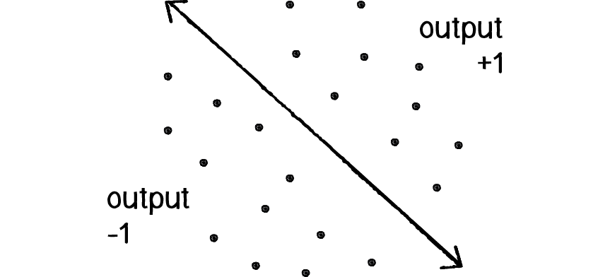
Figure 10.4
Consider a line in two-dimensional space. Points in that space can be classified as living on either one side of the line or the other. While this is a somewhat silly example (since there is clearly no need for a neural network; we can determine on which side a point lies with some simple algebra), it shows how a perceptron can be trained to recognize points on one side versus another.
Let’s say a perceptron has 2 inputs (the x- and y-coordinates of a point). Using a sign activation function, the output will either be -1 or 1—i.e., the input data is classified according to the sign of the output. In the above diagram, we can see how each point is either below the line (-1) or above (+1).
The perceptron itself can be diagrammed as follows:
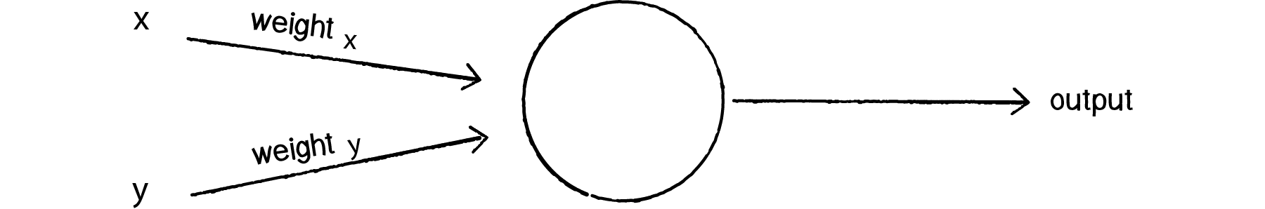
Figure 10.5
We can see how there are two inputs (x and y), a weight for each input (weightx and weighty), as well as a processing neuron that generates the output.
There is a pretty significant problem here, however. Let’s consider the point (0,0). What if we send this point into the perceptron as its input: x = 0 and y = 0? What will the sum of its weighted inputs be? No matter what the weights are, the sum will always be 0! But this can’t be right—after all, the point (0,0) could certainly be above or below various lines in our two-dimensional world.
To avoid this dilemma, our perceptron will require a third input, typically referred to as a bias input. A bias input always has the value of 1 and is also weighted. Here is our perceptron with the addition of the bias:
Figure 10.6
Let’s go back to the point (0,0). Here are our inputs:
0 * weight for x = 0
0 * weight for y = 0
1 * weight for bias = weight for bias
The output is the sum of the above three values, 0 plus 0 plus the bias’s weight. Therefore, the bias, on its own, answers the question as to where (0,0) is in relation to the line. If the bias’s weight is positive, (0,0) is above the line; negative, it is below. It “biases” the perceptron’s understanding of the line’s position relative to (0,0).
10.4 Coding the Perceptron
We’re now ready to assemble the code for a Perceptron class. The only data the perceptron needs to track are the input weights, and we could use an array of floats to store these.
class Perceptron {
float[] weights;
The constructor could receive an argument indicating the number of inputs (in this case three: x, y, and a bias) and size the array accordingly.
Perceptron(int n) {
weights = new float[n];
for (int i = 0; i < weights.length; i++) {
weights[i] = random(-1,1);
}
}
A perceptron needs to be able to receive inputs and generate an output. We can package these requirements into a function called feedforward(). In this example, we’ll have the perceptron receive its inputs as an array (which should be the same length as the array of weights) and return the output as an integer.
int feedforward(float[] inputs) {
float sum = 0;
for (int i = 0; i < weights.length; i++) {
sum += inputs[i]*weights[i];
}
return activate(sum);
}
Presumably, we could now create a Perceptron object and ask it to make a guess for any given point.
Figure 10.7
Perceptron p = new Perceptron(3);float[] point = {50,-12,1};int result = p.feedforward(point);Did the perceptron get it right? At this point, the perceptron has no better than a 50/50 chance of arriving at the right answer. Remember, when we created it, we gave each weight a random value. A neural network isn’t magic. It’s not going to be able to guess anything correctly unless we teach it how to!
To train a neural network to answer correctly, we’re going to employ the method of supervised learning that we described in section 10.1.
With this method, the network is provided with inputs for which there is a known answer. This way the network can find out if it has made a correct guess. If it’s incorrect, the network can learn from its mistake and adjust its weights. The process is as follows:
Provide the perceptron with inputs for which there is a known answer.
Ask the perceptron to guess an answer.
Compute the error. (Did it get the answer right or wrong?)
Adjust all the weights according to the error.
Return to Step 1 and repeat!
Steps 1 through 4 can be packaged into a function. Before we can write the entire function, however, we need to examine Steps 3 and 4 in more detail. How do we define the perceptron’s error? And how should we adjust the weights according to this error?
The perceptron’s error can be defined as the difference between the desired answer and its guess.
ERROR = DESIRED OUTPUT - GUESS OUTPUT
The above formula may look familiar to you. In Chapter 6, we computed a steering force as the difference between our desired velocity and our current velocity.
STEERING = DESIRED VELOCITY - CURRENT VELOCITY
This was also an error calculation. The current velocity acts as a guess and the error (the steering force) tells us how to adjust the velocity in the right direction. In a moment, we’ll see how adjusting the vehicle’s velocity to follow a target is just like adjusting the weights of a neural network to arrive at the right answer.
In the case of the perceptron, the output has only two possible values: +1 or -1. This means there are only three possible errors.
If the perceptron guesses the correct answer, then the guess equals the desired output and the error is 0. If the correct answer is -1 and we’ve guessed +1, then the error is -2. If the correct answer is +1 and we’ve guessed -1, then the error is +2.
| Desired | Guess | Error |
|---|---|---|
-1 |
-1 |
0 |
-1 |
+1 |
-2 |
+1 |
-1 |
+2 |
+1 |
+1 |
0 |
The error is the determining factor in how the perceptron’s weights should be adjusted. For any given weight, what we are looking to calculate is the change in weight, often called Δweight (or “delta” weight, delta being the Greek letter Δ).
NEW WEIGHT = WEIGHT + ΔWEIGHT
Δweight is calculated as the error multiplied by the input.
ΔWEIGHT = ERROR * INPUT
Therefore:
NEW WEIGHT = WEIGHT + ERROR * INPUT
To understand why this works, we can again return to steering. A steering force is essentially an error in velocity. If we apply that force as our acceleration (Δvelocity), then we adjust our velocity to move in the correct direction. This is what we want to do with our neural network’s weights. We want to adjust them in the right direction, as defined by the error.
With steering, however, we had an additional variable that controlled the vehicle’s ability to steer: the maximum force. With a high maximum force, the vehicle was able to accelerate and turn very quickly; with a lower force, the vehicle would take longer to adjust its velocity. The neural network will employ a similar strategy with a variable called the “learning constant.” We’ll add in the learning constant as follows:
NEW WEIGHT = WEIGHT + ERROR * INPUT * LEARNING CONSTANT
Notice that a high learning constant means the weight will change more drastically. This may help us arrive at a solution more quickly, but with such large changes in weight it’s possible we will overshoot the optimal weights. With a small learning constant, the weights will be adjusted slowly, requiring more training time but allowing the network to make very small adjustments that could improve the network’s overall accuracy.
Assuming the addition of a variable c for the learning constant, we can now write a training function for the perceptron following the above steps.
float c = 0.01;
void train(float[] inputs, int desired) {
int guess = feedforward(inputs);
float error = desired - guess;
for (int i = 0; i < weights.length; i++) {
weights[i] += c * error * inputs[i];
}
}We can now see the Perceptron class as a whole.
class Perceptron { float[] weights;
float c = 0.01;
Perceptron(int n) {
weights = new float[n];
for (int i = 0; i < weights.length; i++) {
weights[i] = random(-1,1);
}
}
int feedforward(float[] inputs) {
float sum = 0;
for (int i = 0; i < weights.length; i++) {
sum += inputs[i]*weights[i];
}
return activate(sum);
}
int activate(float sum) {
  if (sum > 0) return 1;
  else return -1;
}
void train(float[] inputs, int desired) {
int guess = feedforward(inputs);
float error = desired - guess;
for (int i = 0; i < weights.length; i++) {
weights[i] += c * error * inputs[i];
}
}
}To train the perceptron, we need a set of inputs with a known answer. We could package this up in a class like so:
class Trainer {
float[] inputs;
int answer;
Trainer(float x, float y, int a) {
inputs = new float[3];
inputs[0] = x;
inputs[1] = y;
inputs[2] = 1;
answer = a;
}
}
Now the question becomes, how do we pick a point and know whether it is above or below a line? Let’s start with the formula for a line, where y is calculated as a function of x:
y = f(x)
In generic terms, a line can be described as:
y = ax + b
Here’s a specific example:
y = 2*x + 1
We can then write a Processing function with this in mind.
float f(float x) {
return 2*x+1;
}
So, if we make up a point:
float x = random(width);
float y = random(height);
How do we know if this point is above or below the line? The line function f(x) gives us the y value on the line for that x position. Let’s call that yline.
float yline = f(x);If the y value we are examining is above the line, it will be less than yline.
Figure 10.8
if (y < yline) { answer = -1;
} else {
answer = 1;
}
We can then make a Trainer object with the inputs and the correct answer.
Trainer t = new Trainer(x, y, answer);Assuming we had a Perceptron object ptron, we could then train it by sending the inputs along with the known answer.
ptron.train(t.inputs,t.answer);Now, it’s important to remember that this is just a demonstration. Remember our Shakespeare-typing monkeys? We asked our genetic algorithm to solve for “to be or not to be”—an answer we already knew. We did this to make sure our genetic algorithm worked properly. The same reasoning applies to this example. We don’t need a perceptron to tell us whether a point is above or below a line; we can do that with simple math. We are using this scenario, one that we can easily solve without a perceptron, to demonstrate the perceptron’s algorithm as well as easily confirm that it is working properly.
Let’s look at how the perceptron works with an array of many training points.
Perceptron ptron;Trainer[] training = new Trainer[2000];
int count = 0;
float f(float x) {
return 2*x+1;
}
void setup() {
size(640, 360);
ptron = new Perceptron(3);
for (int i = 0; i < training.length; i++) {
float x = random(-width/2,width/2);
float y = random(-height/2,height/2);
int answer = 1;
if (y < f(x)) answer = -1;
training[i] = new Trainer(x, y, answer);
}
}
void draw() {
background(255);
translate(width/2,height/2);
ptron.train(training[count].inputs, training[count].answer);
count = (count + 1) % training.length;
for (int i = 0; i < count; i++) {
stroke(0);
int guess = ptron.feedforward(training[i].inputs);
if (guess > 0) noFill();
else fill(0);
ellipse(training[i].inputs[0], training[i].inputs[1], 8, 8);
}
}
10.5 A Steering Perceptron
While classifying points according to their position above or below a line was a useful demonstration of the perceptron in action, it doesn’t have much practical relevance to the other examples throughout this book. In this section, we’ll take the concepts of a perceptron (array of inputs, single output), apply it to steering behaviors, and demonstrate reinforcement learning along the way.
We are now going to take significant creative license with the concept of a neural network. This will allow us to stick with the basics and avoid some of the highly complex algorithms associated with more sophisticated neural networks. Here we’re not so concerned with following rules outlined in artificial intelligence textbooks—we’re just hoping to make something interesting and brain-like.
Remember our good friend the Vehicle class? You know, that one for making objects with a location, velocity, and acceleration? That could obey Newton’s laws with an applyForce() function and move around the window according to a variety of steering rules?
What if we added one more variable to our Vehicle class?
class Vehicle {
Perceptron brain;
PVector location;
PVector velocity;
PVector acceleration;
//etc...
Here’s our scenario. Let’s say we have a Processing sketch with an ArrayList of targets and a single vehicle.
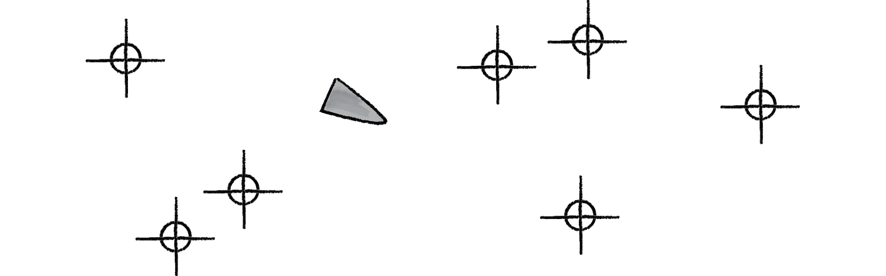
Figure 10.9
Let’s say that the vehicle seeks all of the targets. According to the principles of Chapter 6, we would next write a function that calculates a steering force towards each target, applying each force one at a time to the object’s acceleration. Assuming the targets are an ArrayList of PVector objects, it would look something like:
void seek(ArrayList<PVector> targets) {
for (PVector target : targets) {
PVector force = seek(targets.get(i));
applyForce(force);
}
}
In Chapter 6, we also examined how we could create more dynamic simulations by weighting each steering force according to some rule. For example, we could say that the farther you are from a target, the stronger the force.
void seek(ArrayList<PVector> targets) {
for (PVector target : targets) {
PVector force = seek(targets.get(i));
float d = PVector.dist(target,location);
float weight = map(d,0,width,0,5);
force.mult(weight);
applyForce(force);
}
}
But what if instead we could ask our brain (i.e. perceptron) to take in all the forces as an input, process them according to weights of the perceptron inputs, and generate an output steering force? What if we could instead say:
void seek(ArrayList<PVector> targets) {
PVector[] forces = new PVector[targets.size()];
for (int i = 0; i < forces.length; i++) {
forces[i] = seek(targets.get(i));
}
PVector output = brain.process(forces);
applyForce(output);
}In other words, instead of weighting and accumulating the forces inside our vehicle, we simply pass an array of forces to the vehicle’s “brain” object and allow the brain to weight and sum the forces for us. The output is then applied as a steering force. This opens up a range of possibilities. A vehicle could make decisions as to how to steer on its own, learning from its mistakes and responding to stimuli in its environment. Let’s see how this works.
We can use the line classification perceptron as a model, with one important difference—the inputs are not single numbers, but vectors! Let’s look at how the feedforward() function works in our vehicle’s perceptron, alongside the one from our previous example.
| Vehicle PVector inputs | Line float inputs |
|---|---|
PVector feedforward(PVector[] forces) {
// Sum is a PVector.
PVector sum = new PVector();
for (int i = 0; i < weights.length; i++) {
// Vector addition and multiplication
forces[i].mult(weights[i]);
sum.add(forces[i]);
}
// No activation function
return sum;
}
|
int feedforward(float[] inputs) {
// Sum is a float.
float sum = 0;
for (int i = 0; i < weights.length; i++) {
// Scalar addition and multiplication
sum += inputs[i]*weights[i];
}
// Activation function
    return activate(sum);
  }
|
Note how these two functions implement nearly identical algorithms, with two differences:
Summing PVectors. Instead of a series of numbers added together, each input is a PVector and must be multiplied by the weight and added to a sum according to the mathematical PVector functions.
No activation function. In this case, we’re taking the result and applying it directly as a steering force for the vehicle, so we’re not asking for a simple boolean value that classifies it in one of two categories. Rather, we’re asking for raw output itself, the resulting overall force.
Once the resulting steering force has been applied, it’s time to give feedback to the brain, i.e. reinforcement learning. Was the decision to steer in that particular direction a good one or a bad one? Presumably if some of the targets were predators (resulting in being eaten) and some of the targets were food (resulting in greater health), the network would adjust its weights in order to steer away from the predators and towards the food.
Let’s take a simpler example, where the vehicle simply wants to stay close to the center of the window. We’ll train the brain as follows:
PVector desired = new PVector(width/2,height/2);
PVector error = PVector.sub(desired, location);
brain.train(forces,error);
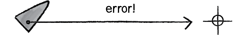
Figure 10.10
Here we are passing the brain a copy of all the inputs (which it will need for error correction) as well as an observation about its environment: a PVector that points from its current location to where it desires to be. This PVector essentially serves as the error—the longer the PVector, the worse the vehicle is performing; the shorter, the better.
The brain can then apply this “error” vector (which has two error values, one for x and one for y) as a means for adjusting the weights, just as we did in the line classification example.
| Training the Vehicle | Training the Line Classifier |
|---|---|
void train(PVector[] forces, PVector error) {
for (int i = 0; i < weights.length; i++) {
weights[i] += c*error.x*forces[i].x;
weights[i] += c*error.y*forces[i].y;
}
}
|
void train(float[] inputs, int desired) {
int guess = feedforward(inputs);
float error = desired - guess;
  for (int i = 0; i < weights.length; i++) {
    weights[i] += c * error * inputs[i];
  }
}
|
Because the vehicle observes its own error, there is no need to calculate one; we can simply receive the error as an argument. Notice how the change in weight is processed twice, once for the error along the x-axis and once for the y-axis.
weights[i] += c*error.x*forces[i].x;
weights[i] += c*error.y*forces[i].y;
We can now look at the Vehicle class and see how the steer function uses a perceptron to control the overall steering force. The new content from this chapter is highlighted.
Example 10.2: Perceptron steering
class Vehicle {
Perceptron brain;
PVector location;
PVector velocity;
PVector acceleration;
float maxforce;
float maxspeed;
Vehicle(int n, float x, float y) {
brain = new Perceptron(n,0.001);
acceleration = new PVector(0,0);
velocity = new PVector(0,0);
location = new PVector(x,y);
maxspeed = 4;
maxforce = 0.1;
}
void update() {
velocity.add(acceleration);
velocity.limit(maxspeed);
location.add(velocity);
acceleration.mult(0);
}
void applyForce(PVector force) {
acceleration.add(force);
}
void steer(ArrayList<PVector> targets) {
    PVector[] forces = new PVector[targets.size()];

    for (int i = 0; i < forces.length; i++) {
      forces[i] = seek(targets.get(i));
    }
PVector result = brain.feedforward(forces);
applyForce(result);
    PVector desired = new PVector(width/2,height/2);
    PVector error = PVector.sub(desired, location);
    brain.train(forces,error);
}
  PVector seek(PVector target) {
    PVector desired = PVector.sub(target,location);
    desired.normalize();
    desired.mult(maxspeed);
    PVector steer = PVector.sub(desired,velocity);
    steer.limit(maxforce);
    return steer;
  }
}
10.6 It’s a “Network,” Remember?
Yes, a perceptron can have multiple inputs, but it is still a lonely neuron. The power of neural networks comes in the networking itself. Perceptrons are, sadly, incredibly limited in their abilities. If you read an AI textbook, it will say that a perceptron can only solve linearly separable problems. What’s a linearly separable problem? Let’s take a look at our first example, which determined whether points were on one side of a line or the other.
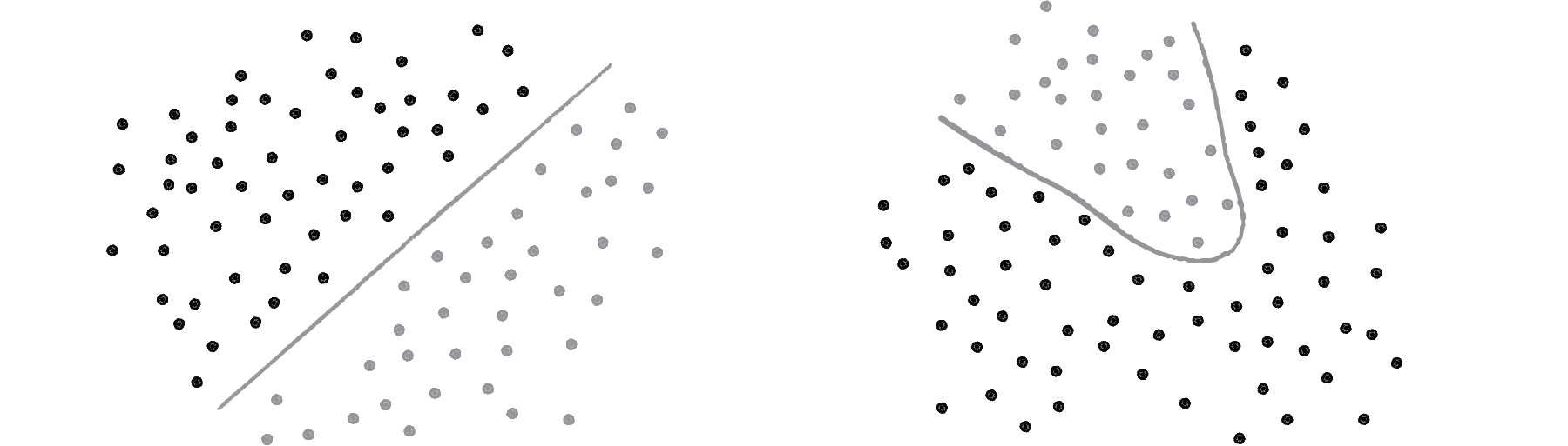
Figure 10.11
On the left of Figure 10.11, we have classic linearly separable data. Graph all of the possibilities; if you can classify the data with a straight line, then it is linearly separable. On the right, however, is non-linearly separable data. You can’t draw a straight line to separate the black dots from the gray ones.
One of the simplest examples of a non-linearly separable problem is XOR, or “exclusive or.” We’re all familiar with AND. For A AND B to be true, both A and B must be true. With OR, either A or B can be true for A OR B to evaluate as true. These are both linearly separable problems. Let’s look at the solution space, a “truth table.”
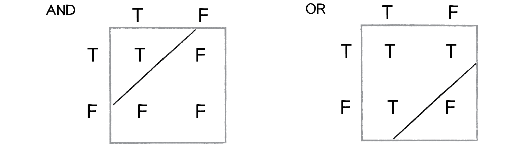
Figure 10.12
See how you can draw a line to separate the true outputs from the false ones?
XOR is the equivalent of OR and NOT AND. In other words, A XOR B only evaluates to true if one of them is true. If both are false or both are true, then we get false. Take a look at the following truth table.

Figure 10.13
This is not linearly separable. Try to draw a straight line to separate the true outputs from the false ones—you can’t!
So perceptrons can’t even solve something as simple as XOR. But what if we made a network out of two perceptrons? If one perceptron can solve OR and one perceptron can solve NOT AND, then two perceptrons combined can solve XOR.
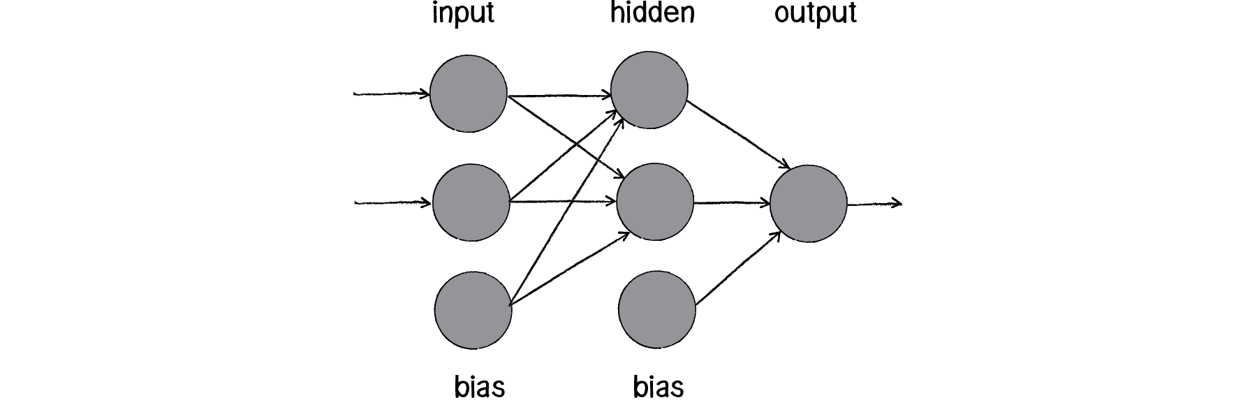
Figure 10.14
The above diagram is known as a multi-layered perceptron, a network of many neurons. Some are input neurons and receive the inputs, some are part of what’s called a “hidden” layer (as they are connected to neither the inputs nor the outputs of the network directly), and then there are the output neurons, from which we read the results.
Training these networks is much more complicated. With the simple perceptron, we could easily evaluate how to change the weights according to the error. But here there are so many different connections, each in a different layer of the network. How does one know how much each neuron or connection contributed to the overall error of the network?
The solution to optimizing weights of a multi-layered network is known as backpropagation. The output of the network is generated in the same manner as a perceptron. The inputs multiplied by the weights are summed and fed forward through the network. The difference here is that they pass through additional layers of neurons before reaching the output. Training the network (i.e. adjusting the weights) also involves taking the error (desired result - guess). The error, however, must be fed backwards through the network. The final error ultimately adjusts the weights of all the connections.
Backpropagation is a bit beyond the scope of this book and involves a fancier activation function (called the sigmoid function) as well as some basic calculus. If you are interested in how backpropagation works, check the book website (and GitHub repository) for an example that solves XOR using a multi-layered feed forward network with backpropagation.
Instead, here we’ll focus on a code framework for building the visual architecture of a network. We’ll make Neuron objects and Connection objects from which a Network object can be created and animated to show the feed forward process. This will closely resemble some of the force-directed graph examples we examined in Chapter 5 (toxiclibs).
10.7 Neural Network Diagrams
Our goal will be to create the following simple network diagram:
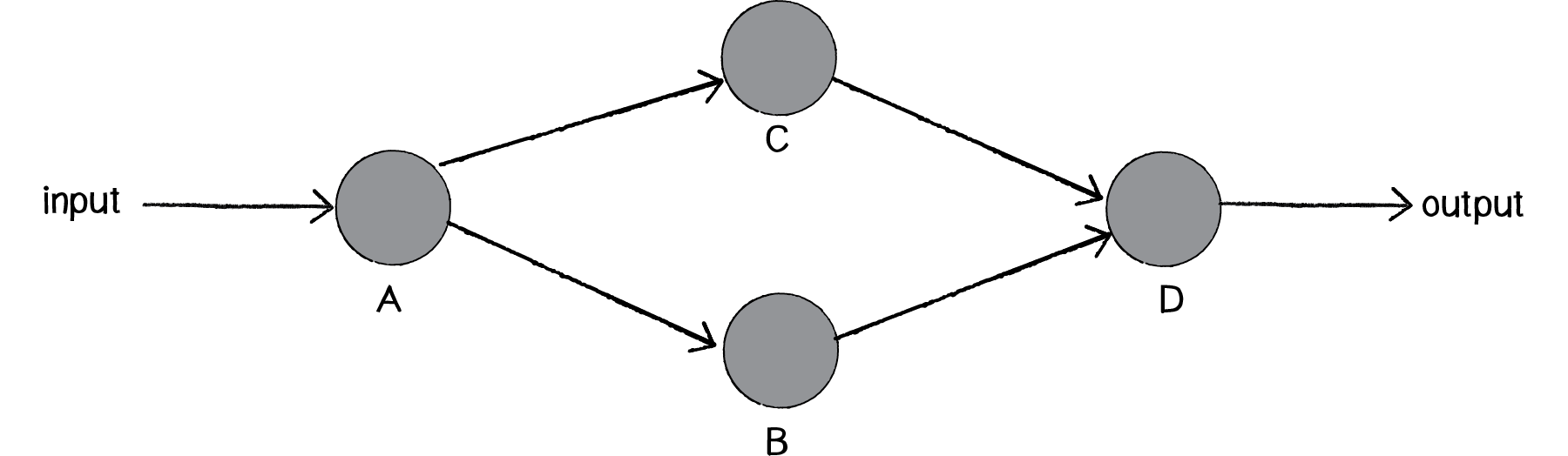
Figure 10.15
The primary building block for this diagram is a neuron. For the purpose of this example, the Neuron class describes an entity with an (x,y) location.
class Neuron {
  PVector location;

  Neuron(float x, float y) {
    location = new PVector(x, y);
  }

  void display() {
    stroke(0);
    fill(0);
    ellipse(location.x, location.y, 16, 16);
  }
}
The Network class can then manage an ArrayList of neurons, as well as have its own location (so that each neuron is drawn relative to the network’s center). This is particle systems 101. We have a single element (a neuron) and a network (a “system” of many neurons).
class Network {
  ArrayList<Neuron> neurons;
  PVector location;

  Network(float x, float y) {
    location = new PVector(x,y);
    neurons = new ArrayList<Neuron>();
  }
  void addNeuron(Neuron n) {
    neurons.add(n);
  }
  void display() {
    pushMatrix();
    translate(location.x, location.y);
    for (Neuron n : neurons) {
      n.display();
    }
    popMatrix();
  }
}Now we can pretty easily make the diagram above.
Network network;

void setup() {
  size(640, 360);
network = new Network(width/2,height/2);
  Neuron a = new Neuron(-200,0);
  Neuron b = new Neuron(0,100);
  Neuron c = new Neuron(0,-100);
  Neuron d = new Neuron(200,0);
  network.addNeuron(a);
  network.addNeuron(b);
  network.addNeuron(c);
  network.addNeuron(d);
}

void draw() {
  background(255);
  network.display();
}
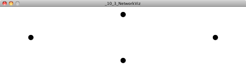
The above yields:
What’s missing, of course, is the connection. We can consider a Connection object to be made up of three elements, two neurons (from Neuron a to Neuron b) and a weight.
class Connection { Neuron a;
Neuron b;
float weight;
Connection(Neuron from, Neuron to,float w) {
weight = w;
a = from;
b = to;
}
void display() {
stroke(0);
strokeWeight(weight*4);
line(a.location.x, a.location.y, b.location.x, b.location.y);
}
}
Once we have the idea of a Connection object, we can write a function (let’s put it inside the Network class) that connects two neurons together—the goal being that in addition to making the neurons in setup(), we can also connect them.
void setup() {
size(640, 360);
network = new Network(width/2,height/2);
Neuron a = new Neuron(-200,0);
Neuron b = new Neuron(0,100);
Neuron c = new Neuron(0,-100);
Neuron d = new Neuron(200,0);
network.connect(a,b);
network.connect(a,c);
network.connect(b,d);
network.connect(c,d);
network.addNeuron(a);
network.addNeuron(b);
network.addNeuron(c);
network.addNeuron(d);
}
The Network class therefore needs a new function called connect(), which makes a Connection object between the two specified neurons.
void connect(Neuron a, Neuron b) { Connection c = new Connection(a, b, random(1));
// But what do we do with the Connection object?
}
Presumably, we might think that the Network should store an ArrayList of connections, just like it stores an ArrayList of neurons. While useful, in this case such an ArrayList is not necessary and is missing an important feature that we need. Ultimately we plan to “feed forward" the neurons through the network, so the Neuron objects themselves must know to which neurons they are connected in the “forward” direction. In other words, each neuron should have its own list of Connection objects. When a connects to b, we want a to store a reference of that connection so that it can pass its output to b when the time comes.
void connect(Neuron a, Neuron b) {
Connection c = new Connection(a, b, random(1));
a.addConnection(c);
}
In some cases, we also might want Neuron b to know about this connection, but in this particular example we are only going to pass information in one direction.
For this to work, we have to add an ArrayList of connections to the Neuron class. Then we implement the addConnection() function that stores the connection in that ArrayList.
class Neuron {
PVector location;
ArrayList<Connection> connections;
Neuron(float x, float y) {
location = new PVector(x, y);
connections = new ArrayList<Connection>();
}
void addConnection(Connection c) {
connections.add(c);
}
The neuron’s display() function can draw the connections as well. And finally, we have our network diagram.
Example 10.3: Neural network diagram
void display() {
stroke(0);
strokeWeight(1);
fill(0);
ellipse(location.x, location.y, 16, 16);
for (Connection c : connections) {
c.display();
}
}
}
10.8 Animating Feed Forward
An interesting problem to consider is how to visualize the flow of information as it travels throughout a neural network. Our network is built on the feed forward model, meaning that an input arrives at the first neuron (drawn on the lefthand side of the window) and the output of that neuron flows across the connections to the right until it exits as output from the network itself.
Our first step is to add a function to the network to receive this input, which we’ll make a random number between 0 and 1.
void setup() {
network.feedforward(random(1));
}
The network, which manages all the neurons, can choose to which neurons it should apply that input. In this case, we’ll do something simple and just feed a single input into the first neuron in the ArrayList, which happens to be the left-most one.
class Network {
void feedforward(float input) {
Neuron start = neurons.get(0);
start.feedforward(input);
}
What did we do? Well, we made it necessary to add a function called feedforward() in the Neuron class that will receive the input and process it.
class Neuron
void feedforward(float input) {
}
If you recall from working with our perceptron, the standard task that the processing unit performs is to sum up all of its inputs. So if our Neuron class adds a variable called sum, it can simply accumulate the inputs as they are received.
class Neuron
int sum = 0;
void feedforward(float input) {
sum += input;
}
The neuron can then decide whether it should “fire,” or pass an output through any of its connections to the next layer in the network. Here we can create a really simple activation function: if the sum is greater than 1, fire!
void feedforward(float input) {
sum += input;
if (sum > 1) {
fire();
sum = 0;
}
}
Now, what do we do in the fire() function? If you recall, each neuron keeps track of its connections to other neurons. So all we need to do is loop through those connections and feedforward() the neuron’s output. For this simple example, we’ll just take the neuron’s sum variable and make it the output.
void fire() {
for (Connection c : connections) {
c.feedforward(sum);
}
}
Here’s where things get a little tricky. After all, our job here is not to actually make a functioning neural network, but to animate a simulation of one. If the neural network were just continuing its work, it would instantly pass those inputs (multiplied by the connection’s weight) along to the connected neurons. We’d say something like:
class Connection {
void feedforward(float val) {
b.feedforward(val*weight);
}
But this is not what we want. What we want to do is draw something that we can see traveling along the connection from Neuron a to Neuron b.
Let’s first think about how we might do that. We know the location of Neuron a; it’s the PVector a.location. Neuron b is located at b.location. We need to start something moving from Neuron a by creating another PVector that will store the path of our traveling data.
PVector sender = a.location.get();Once we have a copy of that location, we can use any of the motion algorithms that we’ve studied throughout this book to move along this path. Here—let’s pick something very simple and just interpolate from a to b.
sender.x = lerp(sender.x, b.location.x, 0.1);
sender.y = lerp(sender.y, b.location.y, 0.1);
Along with the connection’s line, we can then draw a circle at that location:
stroke(0);
line(a.location.x, a.location.y, b.location.x, b.location.y);
fill(0);
ellipse(sender.x, sender.y, 8, 8);
This resembles the following:

Figure 10.16
OK, so that’s how we might move something along the connection. But how do we know when to do so? We start this process the moment the Connection object receives the “feedforward” signal. We can keep track of this process by employing a simple boolean to know whether the connection is sending or not. Before, we had:
void feedforward(float val) {
b.feedforward(val*weight);
}
Now, instead of sending the value on straight away, we’ll trigger an animation:
class Connection {
boolean sending = false;
PVector sender;
float output;
void feedforward(float val) {
sending = true; sender = a.location.get(); output = val*weight;
}
Notice how our Connection class now needs three new variables. We need a boolean “sending” that starts as false and that will track whether or not the connection is actively sending (i.e. animating). We need a PVector “sender” for the location where we’ll draw the traveling dot. And since we aren’t passing the output along this instant, we’ll need to store it in a variable that will do the job later.
The feedforward() function is called the moment the connection becomes active. Once it’s active, we’ll need to call another function continuously (each time through draw()), one that will update the location of the traveling data.
void update() {
if (sending) {
sender.x = lerp(sender.x, b.location.x, 0.1);
sender.y = lerp(sender.y, b.location.y, 0.1);
}
}
We’re missing a key element, however. We need to check if the sender has arrived at location b, and if it has, feed forward that output to the next neuron.
void update() {
if (sending) {
sender.x = lerp(sender.x, b.location.x, 0.1);
sender.y = lerp(sender.y, b.location.y, 0.1);
float d = PVector.dist(sender, b.location);
if (d < 1) {
b.feedforward(output);
sending = false;
}
}
}
Let’s look at the Connection class all together, as well as our new draw() function.
Example 10.4: Animating a neural network diagram
void draw() {
background(255);
network.update();
network.display();
if (frameCount % 30 == 0) {
network.feedforward(random(1));
}
}
class Connection {
float weight;
  Neuron a;
  Neuron b;
boolean sending = false;
PVector sender;
float output = 0;
Connection(Neuron from, Neuron to, float w) {
weight = w;
a = from;
b = to;
}
void feedforward(float val) {
output = val*weight;
sender = a.location.get();
sending = true;
}
void update() {
if (sending) {
sender.x = lerp(sender.x, b.location.x, 0.1);
sender.y = lerp(sender.y, b.location.y, 0.1);
float d = PVector.dist(sender, b.location);
if (d < 1) {
b.feedforward(output);
sending = false;
  }
}
}
void display() {
stroke(0);
strokeWeight(1+weight*4);
line(a.location.x, a.location.y, b.location.x, b.location.y);
if (sending) {
fill(0);
strokeWeight(1);
ellipse(sender.x, sender.y, 16, 16);
    }
  }
}
Exercise 10.5
The network in the above example was manually configured by setting the location of each neuron and its connections with hard-coded values. Rewrite this example to generate the network’s layout via an algorithm. Can you make a circular network diagram? A random one? An example of a multi-layered network is below.
Exercise 10.6
Rewrite the example so that each neuron keeps track of its forward and backward connections. Can you feed inputs through the network in any direction?
Exercise 10.7
Instead of lerp(), use moving bodies with steering forces to visualize the flow of information in the network.
The Ecosystem Project
Step 10 Exercise:
Try incorporating the concept of a “brain” into your creatures.
Use reinforcement learning in the creatures’ decision-making process.
Create a creature that features a visualization of its brain as part of its design (even if the brain itself is not functional).
Can the ecosystem as a whole emulate the brain? Can elements of the environment be neurons and the creatures act as inputs and outputs?
The end
If you’re still reading, thank you! You’ve reached the end of the book. But for as much material as this book contains, we’ve barely scratched the surface of the world we inhabit and of techniques for simulating it. It’s my intention for this book to live as an ongoing project, and I hope to continue adding new tutorials and examples to the book’s website as well as expand and update the printed material. Your feedback is truly appreciated, so please get in touch via email at (daniel@shiffman.net) or by contributing to the GitHub repository, in keeping with the open-source spirit of the project. Share your work. Keep in touch. Let’s be two with nature.

