3.1 Angles

OK. Before we can do any of this stuff, we need to make sure we understand what it means to be an angle in Processing. If you have experience with Processing, you’ve undoubtedly encountered this issue while using the rotate() function to rotate and spin objects.

The first order of business is to cover radians and degrees. You’re probably familiar with the concept of an angle in degrees. A full rotation goes from 0 to 360 degrees. 90 degrees (a right angle) is 1/4th of 360, shown below as two perpendicular lines.

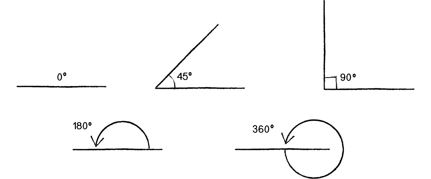
Figure 3.1

It’s fairly intuitive for us to think of angles in terms of degrees. For example, the square in Figure 3.2 is rotated 45 degrees around its center.

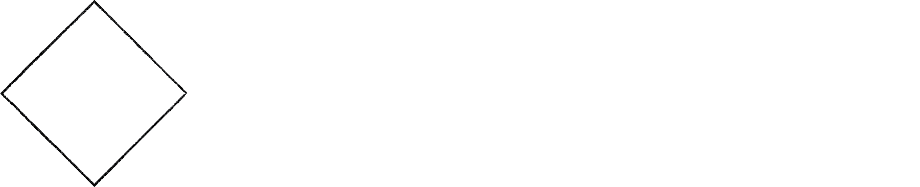
Figure 3.3

Processing, however, requires angles to be specified in radians. A radian is a unit of measurement for angles defined by the ratio of the length of the arc of a circle to the radius of that circle. One radian is the angle at which that ratio equals one (see Figure 3.1). 180 degrees = PI radians, 360 degrees = 2*PI radians, 90 degrees = PI/2 radians, etc.

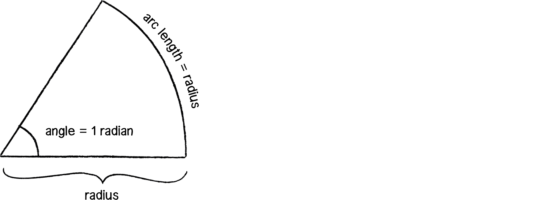
Figure 3.3

The formula to convert from degrees to radians is:

radians = 2 * PI * (degrees / 360)

Thankfully, if we prefer to think in degrees but code with radians, Processing makes this easy. The radians() function will automatically convert values from degrees to radians, and the constants PI and TWO_PI provide convenient access to these commonly used numbers (equivalent to 180 and 360 degrees, respectively). The following code, for example, will rotate shapes by 60 degrees.

float angle = radians(60);
rotate(angle);

If you are not familiar with how rotation is implemented in Processing, I would suggest this tutorial: Processing - Transform 2D.

3.2 Angular Motion

Remember all this stuff?

location = location + velocity
velocity = velocity + acceleration

The stuff we dedicated almost all of Chapters 1 and 2 to? Well, we can apply exactly the same logic to a rotating object.

angle = angle + angular velocity
angular velocity = angular velocity + angular acceleration

In fact, the above is actually simpler than what we started with because an angle is a scalar quantity—a single number, not a vector!

Using the answer from Exercise 3.1 above, let’s say we wanted to rotate a baton in Processing by some angle. We would have code like:

  translate(width/2,height/2);
  rotate(angle);
  line(-50,0,50,0);
  ellipse(50,0,8,8);
  ellipse(-50,0,8,8);

Adding in our principles of motion brings us to the following example.

Example 3.1: Angular motion using rotate()

float angle = 0;

float aVelocity = 0;

float aAcceleration = 0.001;
 
void setup() {
  size(640,360);
}
 
void draw() {
  background(255);
 
  fill(175);
  stroke(0);
  rectMode(CENTER);
  translate(width/2,height/2);
  rotate(angle);
  line(-50,0,50,0);
  ellipse(50,0,8,8);
  ellipse(-50,0,8,8);
 

  aVelocity += aAcceleration;

  angle += aVelocity;
}

The baton starts onscreen with no rotation and then spins faster and faster as the angle of rotation accelerates.

This idea can be incorporated into our Mover object. For example, we can add the variables related to angular motion to our Mover.

class Mover {
 
  PVector location;
  PVector velocity;
  PVector acceleration;
  float mass;
 
  float angle = 0;
  float aVelocity = 0;
  float aAcceleration = 0;

And then in update(), we update both location and angle according to the same algorithm!

 void update() {
 

    velocity.add(acceleration);
    location.add(velocity);

    aVelocity += aAcceleration;
    angle += aVelocity;

 
    acceleration.mult(0);
  }

Of course, for any of this to matter, we also would need to rotate the object when displaying it.

  void display() {
    stroke(0);
    fill(175,200);
    rectMode(CENTER);

    pushMatrix();
 

    translate(location.x,location.y);

    rotate(angle);
    rect(0,0,mass*16,mass*16);
    popMatrix();
  }

Now, if we were to actually go ahead and run the above code, we wouldn’t see anything new. This is because the angular acceleration (float aAcceleration = 0;) is initialized to zero. For the object to rotate, we need to give it an acceleration! Certainly, we could hard-code in a different number.

float aAcceleration = 0.01;

However, we can produce a more interesting result by dynamically assigning an angular acceleration according to forces in the environment. Now, we could head far down this road, trying to model the physics of angular acceleration using the concepts of torque and moment of inertia. Nevertheless, this level of simulation is beyond the scope of this book. (We will see more about modeling angular acceleration with a pendulum later in this chapter, as well as look at how Box2D realistically models rotational motion in Chapter 5.)

For now, a quick and dirty solution will do. We can produce reasonable results by simply calculating angular acceleration as a function of the object’s acceleration vector. Here’s one such example:

    aAcceleration = acceleration.x;

Yes, this is completely arbitrary. But it does do something. If the object is accelerating to the right, its angular rotation accelerates in a clockwise direction; acceleration to the left results in a counterclockwise rotation. Of course, it’s important to think about scale in this case. The x component of the acceleration vector might be a quantity that’s too large, causing the object to spin in a way that looks ridiculous or unrealistic. So dividing the x component by some value, or perhaps constraining the angular velocity to a reasonable range, could really help. Here’s the entire update() function with these tweaks added.

Example 3.2: Forces with (arbitrary) angular motion

  void update() {
 
    velocity.add(acceleration);
    location.add(velocity);
 

    aAcceleration = acceleration.x / 10.0;
    aVelocity += aAcceleration;

    aVelocity = constrain(aVelocity,-0.1,0.1);
    angle += aVelocity;
 
    acceleration.mult(0);
  }

3.3 Trigonometry

I think it may be time. We’ve looked at angles, we’ve spun an object. It’s time for: sohcahtoa. Yes, sohcahtoa. This seemingly nonsensical word is actually the foundation for a lot of computer graphics work. A basic understanding of trigonometry is essential if you want to calculate an angle, figure out the distance between points, work with circles, arcs, or lines. And sohcahtoa is a mnemonic device (albeit a somewhat absurd one) for what the trigonometric functions sine, cosine, and tangent mean.

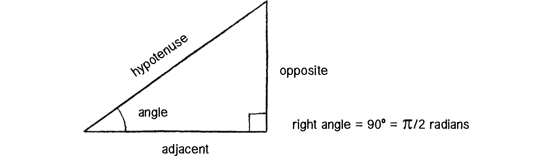
Figure 3.4

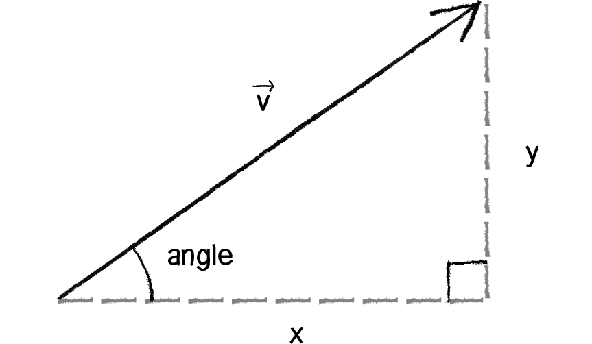
Figure 3.5

Take a look at Figure 3.4 again. There’s no need to memorize it, but make sure you feel comfortable with it. Draw it again yourself. Now let’s draw it a slightly different way (Figure 3.5).

See how we create a right triangle out of a vector? The vector arrow itself is the hypotenuse and the components of the vector (x and y) are the sides of the triangle. The angle is an additional means for specifying the vector’s direction (or “heading”).

Because the trigonometric functions allow us to establish a relationship between the components of a vector and its direction + magnitude, they will prove very useful throughout this book. We’ll begin by looking at an example that requires the tangent function.

3.4 Pointing in the Direction of Movement

Let’s go all the way back to Example 1.10, which features a Mover object accelerating towards the mouse.

You might notice that almost all of the shapes we’ve been drawing so far are circles. This is convenient for a number of reasons, one of which is that we don’t have to consider the question of rotation. Rotate a circle and, well, it looks exactly the same. However, there comes a time in all motion programmers’ lives when they want to draw something on the screen that points in the direction of movement. Perhaps you are drawing an ant, or a car, or a spaceship. And when we say "point in the direction of movement," what we are really saying is “rotate according to the velocity vector.” Velocity is a vector, with an x and a y component, but to rotate in Processing we need an angle, in radians. Let’s draw our trigonometry diagram one more time, with an object’s velocity vector (Figure 3.6).

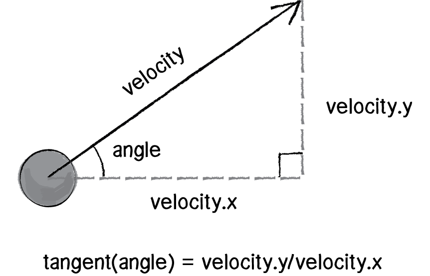
Figure 3.6

OK. We know that the definition of tangent is:

${\displaystyle tangent\left(angle\right)=\frac{{velocity}_y}{{velocity}_x}}$

The problem with the above is that we know velocity, but we don’t know the angle. We have to solve for the angle. This is where a special function known as inverse tangent comes in, sometimes referred to as arctangent or tan^-1. (There is also an inverse sine and an inverse cosine.)

If the tangent of some value a equals some value b, then the inverse tangent of b equals a. For example:

See how that is the inverse? The above now allows us to solve for the angle:

Now that we have the formula, let’s see where it should go in our mover’s display() function. Notice that in Processing, the function for arctangent is called atan().

  void display() {

    float angle = atan(velocity.y/velocity.x);
 
    stroke(0);
    fill(175);
    pushMatrix();
    rectMode(CENTER);
    translate(location.x,location.y);

    rotate(angle);
    rect(0,0,30,10);
    popMatrix();
  }

Now the above code is pretty darn close, and almost works. We still have a big problem, though. Let’s consider the two velocity vectors depicted below.

Figure 3.7

Though superficially similar, the two vectors point in quite different directions—opposite directions, in fact! However, if we were to apply our formula to solve for the angle to each vector…

V1 ⇒ angle = atan(-4/3) = atan(-1.25) = -0.9272952 radians = -53 degrees
V2 ⇒ angle = atan(4/-3) = atan(-1.25) = -0.9272952 radians = -53 degrees

…we get the same angle for each vector. This can’t be right for both; the vectors point in opposite directions! The thing is, this is a pretty common problem in computer graphics. Rather than simply using atan() along with a bunch of conditional statements to account for positive/negative scenarios, Processing (along with pretty much all programming environments) has a nice function called atan2() that does it for you.

Example 3.3: Pointing in the direction of motion

  void display() {

    float angle = atan2(velocity.y,velocity.x);
 
    stroke(0);
    fill(175);
    pushMatrix();
    rectMode(CENTER);
    translate(location.x,location.y);

    rotate(angle);
    rect(0,0,30,10);
    popMatrix();
  }

To simplify this even further, the PVector class itself provides a function called heading(), which takes care of calling atan2() for you so you can get the 2D direction angle, in radians, for any Processing PVector.

    float angle = velocity.heading();

3.5 Polar vs. Cartesian Coordinates

Any time we display a shape in Processing, we have to specify a pixel location, a set of x and y coordinates. These coordinates are known as Cartesian coordinates, named for René Descartes, the French mathematician who developed the ideas behind Cartesian space.

Another useful coordinate system known as polar coordinates describes a point in space as an angle of rotation around the origin and a radius from the origin. Thinking about this in terms of a vector:

Cartesian coordinate—the x,y components of a vector
Polar coordinate—the magnitude (length) and direction (angle) of a vector

Processing’s drawing functions, however, don’t understand polar coordinates. Whenever we want to display something in Processing, we have to specify locations as (x,y) Cartesian coordinates. However, sometimes it is a great deal more convenient for us to think in polar coordinates when designing. Happily for us, with trigonometry we can convert back and forth between polar and Cartesian, which allows us to design with whatever coordinate system we have in mind but always draw with Cartesian coordinates.

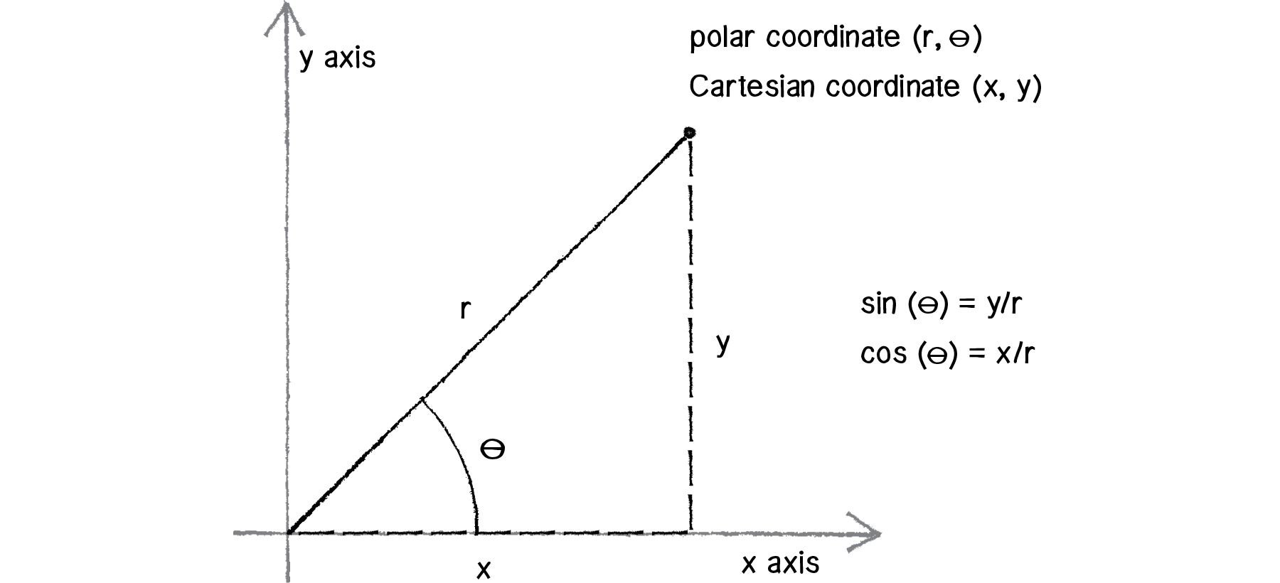
Figure 3.8: The Greek letter θ (theta) is often used to denote an angle. Since a polar coordinate is conventionally referred to as (r, θ), we’ll use theta as a variable name when referring to an angle.

sine(theta)   = y/r   →   y = r * sine(theta)
cosine(theta) = x/r   →   x = r * cosine(theta)

For example, if r is 75 and theta is 45 degrees (or PI/4 radians), we can calculate x and y as below. The functions for sine and cosine in Processing are sin() and cos(), respectively. They each take one argument, an angle measured in radians.

float r = 75;
float theta = PI / 4;

float x = r * cos(theta);
float y = r * sin(theta);

This type of conversion can be useful in certain applications. For example, to move a shape along a circular path using Cartesian coordinates is not so easy. With polar coordinates, on the other hand, it’s simple: increment the angle!

Here’s how it is done with global variables r and theta.

Example 3.4: Polar to Cartesian

float r = 75;
float theta = 0;
 
void setup() {
  size(640,360);
  background(255);
}
 
void draw() {
 

  float x = r * cos(theta);
  float y = r * sin(theta);

 
  noStroke();
  fill(0);
  ellipse(x+width/2, y+height/2, 16, 16);
 
  theta += 0.01;
}

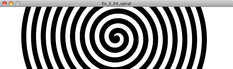
Exercise 3.4

Using Example 3.4 as a basis, draw a spiral path. Start in the center and move outwards. Note that this can be done by only changing one line of code and adding one line of code!

3.6 Oscillation Amplitude and Period

Are you amazed yet? We’ve seen some pretty great uses of tangent (for finding the angle of a vector) and sine and cosine (for converting from polar to Cartesian coordinates). We could stop right here and be satisfied. But we’re not going to. This is only the beginning. What sine and cosine can do for you goes beyond mathematical formulas and right triangles.

Let’s take a look at a graph of the sine function, where y = sine(x).

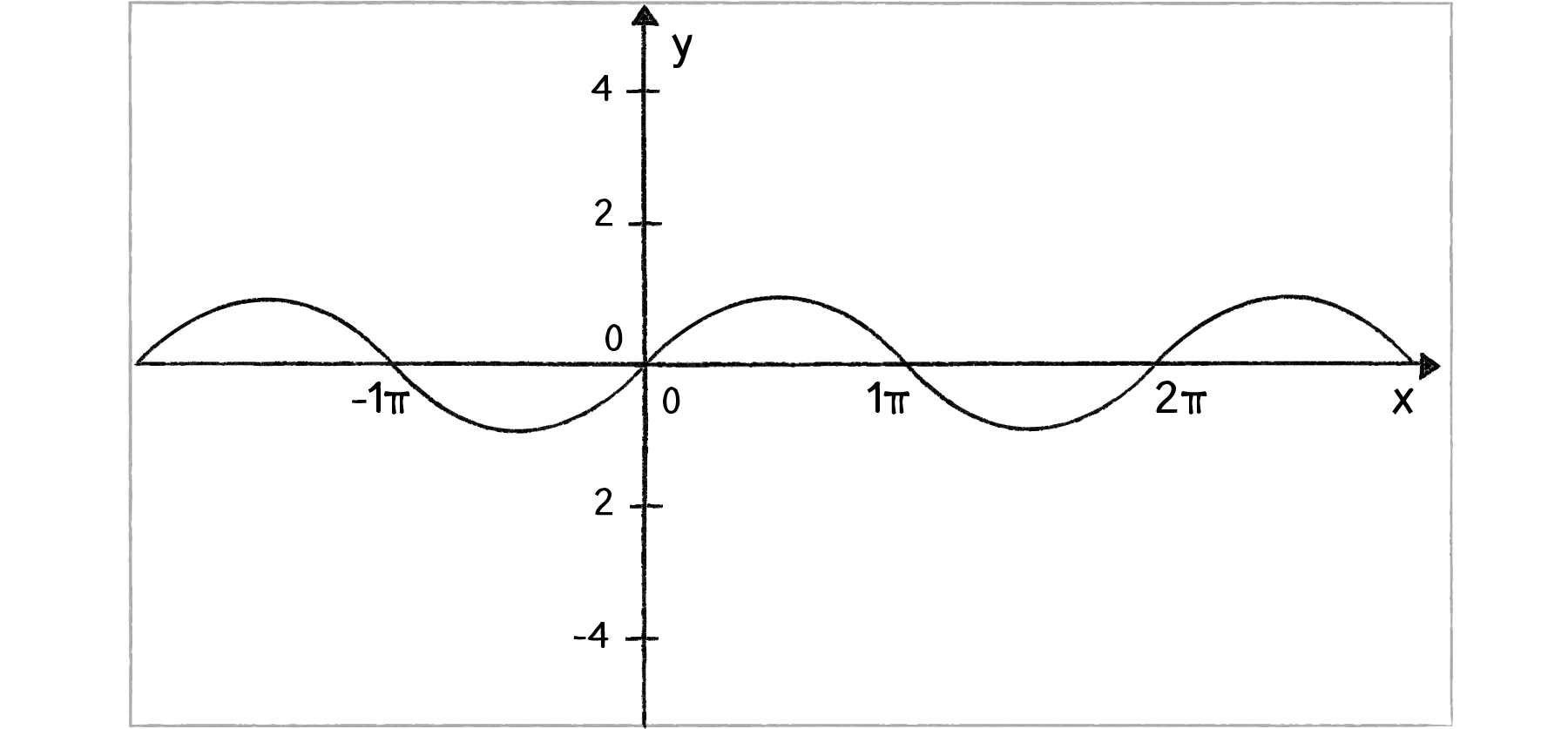
Figure 3.9: y = sine(x)

You’ll notice that the output of the sine function is a smooth curve alternating between –1 and 1. This type of a behavior is known as oscillation, a periodic movement between two points. Plucking a guitar string, swinging a pendulum, bouncing on a pogo stick—these are all examples of oscillating motion.

And so we happily discover that we can simulate oscillation in a Processing sketch by assigning the output of the sine function to an object’s location. Note that this will follow the same methodology we applied to Perlin noise in the Introduction.

Let’s begin with a really basic scenario. We want a circle to oscillate from the left side to the right side of a Processing window.

This is what is known as simple harmonic motion (or, to be fancier, “the periodic sinusoidal oscillation of an object”). It’s going to be a simple program to write, but before we get into the code, let’s familiarize ourselves with some of the terminology of oscillation (and waves).

Simple harmonic motion can be expressed as any location (in our case, the x location) as a function of time, with the following two elements:

Looking at the graph of sine (Figure 3.9), we can see that the amplitude is 1 and the period is TWO_PI; the output of sine never rises above 1 or below -1; and every TWO_PI radians (or 360 degrees) the wave pattern repeats.

Now, in the Processing world we live in, what is amplitude and what is period? Amplitude can be measured rather easily in pixels. In the case of a window 200 pixels wide, we would oscillate from the center 100 pixels to the right and 100 pixels to the left. Therefore:

float amplitude = 100;

Period is the amount of time it takes for one cycle, but what is time in our Processing world? I mean, certainly we could say we want the circle to oscillate every three seconds. And we could track the milliseconds—using millis() —in Processing and come up with an elaborate algorithm for oscillating an object according to real-world time. But for us, real-world time doesn’t really matter. The real measure of time in Processing is in frames. The oscillating motion should repeat every 30 frames, or 50 frames, or 1000 frames, etc.

float period = 120;

Once we have the amplitude and period, it’s time to write a formula to calculate x as a function of time, which we now know is the current frame count.

float x = amplitude * cos(TWO_PI * frameCount / period);

Let’s dissect the formula a bit more and try to understand each component. The first is probably the easiest. Whatever comes out of the cosine function we multiply by amplitude. We know that cosine will oscillate between -1 and 1. If we take that value and multiply it by amplitude then we’ll get the desired result: a value oscillating between -amplitude and amplitude. (Note: this is also a place where we could use Processing’s map() function to map the output of cosine to a custom range.)

Now, let’s look at what is inside the cosine function:

TWO_PI * frameCount / period

What’s going on here? Let’s start with what we know. We know that cosine will repeat every 2*PI radians—i.e. it will start at 0 and repeat at 2*PI, 4*PI, 6*PI, etc. If the period is 120, then we want the oscillating motion to repeat when the frameCount is at 120 frames, 240 frames, 360 frames, etc. frameCount is really the only variable; it starts at 0 and counts upward. Let’s take a look at what the formula yields with those values.

frameCount divided by period tells us how many cycles we’ve completed—are we halfway through the first cycle? Have we completed two cycles? By multiplying that number by TWO_PI, we get the result we want, since TWO_PI is the number of radians required for one cosine (or sine) to complete one cycle.

Wrapping this all up, here’s the Processing example that oscillates the x location of a circle with an amplitude of 100 pixels and a period of 120 frames.

Example 3.5: Simple Harmonic Motion

void setup() {
  size(640,360);
}
 
void draw() {
  background(255);
 
  float period = 120;
  float amplitude = 100;

  float x = amplitude * cos(TWO_PI * frameCount / period);
  stroke(0);
  fill(175);
  translate(width/2,height/2);
  line(0,0,x,0);
  ellipse(x,0,20,20);
}

It’s also worth mentioning the term frequency: the number of cycles per time unit. Frequency is equal to 1 divided by period. If the period is 120 frames, then only 1/120th of a cycle is completed in one frame, and so frequency = 1/120. In the above example, we simply chose to define the rate of oscillation in terms of period and therefore did not need a variable for frequency.

3.7 Oscillation with Angular Velocity

An understanding of the concepts of oscillation, amplitude, and frequency/period is often required in the course of simulating real-world behaviors. However, there is a slightly easier way to rewrite the above example with the same result. Let’s take one more look at our oscillation formula:

float x = amplitude * cos(TWO_PI * frameCount / period);

And let’s rewrite it a slightly different way:

float x = amplitude * cos ( some value that increments slowly );

If we care about precisely defining the period of oscillation in terms of frames of animation, we might need the formula the way we first wrote it, but we can just as easily rewrite our example using the concept of angular velocity (and acceleration) from section 3.2. Assuming:

float angle = 0;
float aVelocity = 0.05;

in draw(), we can simply say:

angle += aVelocity;
float x = amplitude * cos(angle);

angle is our “some value that increments slowly.”

Example 3.6: Simple Harmonic Motion II

float angle = 0;
float aVelocity = 0.05;
 
void setup() {
  size(640,360);
}
 
void draw() {
  background(255);
 
  float amplitude = 100;
  float x = amplitude * cos(angle);

  angle += aVelocity;
 
  ellipseMode(CENTER);
  stroke(0);
  fill(175);
  translate(width/2,height/2);
  line(0,0,x,0);
  ellipse(x,0,20,20);
}

Just because we’re not referencing it directly doesn’t mean that we’ve eliminated the concept of period. After all, the greater the angular velocity, the faster the circle will oscillate (therefore lowering the period). In fact, the number of times it takes to add up the angular velocity to get to TWO_PI is the period or:

period = TWO_PI / angular velocity

Let’s expand this example a bit more and create an Oscillator class. And let’s assume we want the oscillation to happen along both the x-axis (as above) and the y-axis. To do this, we’ll need two angles, two angular velocities, and two amplitudes (one for each axis). Another perfect opportunity for PVector!

Example 3.7: Oscillator objects

class Oscillator  {
 

  PVector angle;
  PVector velocity;
  PVector amplitude;
 
  Oscillator()  {
    angle = new PVector();
    velocity = new PVector(random(-0.05,0.05),random(-0.05,0.05));

    amplitude = new PVector(random(width/2),random(height/2));
  }
 
  void oscillate()  {
    angle.add(velocity);
  }
 
  void display()  {

    float x = sin(angle.x)*amplitude.x;

    float y = sin(angle.y)*amplitude.y;
 
    pushMatrix();
    translate(width/2,height/2);
    stroke(0);
    fill(175);

    line(0,0,x,y);
    ellipse(x,y,16,16);
    popMatrix();
  }
}

3.8 Waves

If you’re saying to yourself, “Um, this is all great and everything, but what I really want is to draw a wave onscreen,” well, then, the time has come. The thing is, we’re about 90% there. When we oscillate a single circle up and down according to the sine function, what we are doing is looking at a single point along the x-axis of a wave pattern. With a little panache and a for loop, we can place a whole bunch of these oscillating circles next to each other.

This wavy pattern could be used in the design of the body or appendages of a creature, as well as to simulate a soft surface (such as water).

Here, we’re going to encounter the same questions of amplitude (height of pattern) and period. Instead of period referring to time, however, since we’re looking at the full wave, we can talk about period as the width (in pixels) of a full wave cycle. And just as with simple oscillation, we have the option of computing the wave pattern according to a precise period or simply following the model of angular velocity.

Let’s go with the simpler case, angular velocity. We know we need to start with an angle, an angular velocity, and an amplitude:

float angle = 0;
float angleVel = 0.2;
float amplitude = 100;

Then we’re going to loop through all of the x values where we want to draw a point of the wave. Let’s say every 24 pixels for now. In that loop, we’re going to want to do three things:

  for (int x = 0; x <= width; x += 24) {
 

    float y = amplitude*sin(angle);
 

    ellipse(x,y+height/2,48,48);
 

    angle += angleVel;
  }

Let’s look at the results with different values for angleVel:

Notice how, although we’re not precisely computing the period of the wave, the higher the angular velocity, the shorter the period. It’s also worth noting that as the period becomes shorter, it becomes more and more difficult to make out the wave itself as the distance between the individual points increases. One option we have is to use beginShape() and endShape() to connect the points with a line.

Example 3.8: Static wave drawn as a continuous line

float angle = 0;
float angleVel = 0.2;
float amplitude = 100;
 
size(400,200);
background(255);
 
stroke(0);
strokeWeight(2);
noFill();
 
beginShape();
for (int x = 0; x <= width; x += 5) {

  float y = map(sin(angle),-1,1,0,height);

  vertex(x,y);
  angle +=angleVel;
}
endShape();

You may have noticed that the above example is static. The wave never changes, never undulates. This additional step is a bit tricky. Your first instinct might be to say: “Hey, no problem, we’ll just let theta be a global variable and let it increment from one cycle through draw() to another.”

While it’s a nice thought, it doesn’t work. If you look at the wave, the righthand edge doesn’t match the lefthand; where it ends in one cycle of draw() can’t be where it starts in the next. Instead, what we need to do is have a variable dedicated entirely to tracking what value of angle the wave should start with. This angle (which we’ll call startAngle) increments with its own angular velocity.

Example 3.9: The Wave

float startAngle = 0;
float angleVel = 0.1;
 
void setup() {
  size(400,200);
}
 
void draw() {
  background(255);
 

float angle = startAngle;

 
  for (int x = 0; x <= width; x += 24) {
    float y = map(sin(angle),-1,1,0,height);
    stroke(0);
    fill(0,50);
    ellipse(x,y,48,48);
    angle += angleVel;
  }
}

3.9 Trigonometry and Forces: The Pendulum

Do you miss Newton’s laws of motion? I know I sure do. Well, lucky for you, it’s time to bring it all back home. After all, it’s been nice learning about triangles and tangents and waves, but really, the core of this book is about simulating the physics of moving bodies. Let’s take a look at how trigonometry can help us with this pursuit.

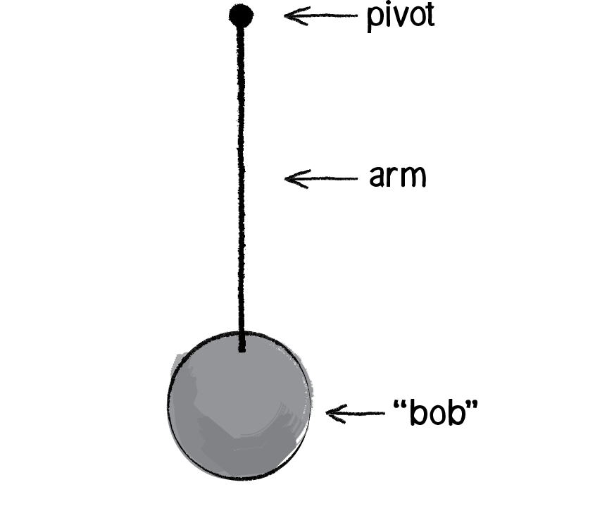
Figure 3.10

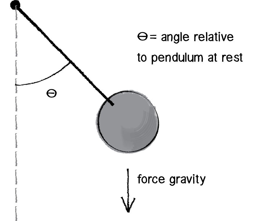
Figure 3.11

A pendulum is a bob suspended from a pivot. Obviously a real-world pendulum would live in a 3D space, but we’re going to look at a simpler scenario, a pendulum in a 2D space—a Processing window (see Figure 3.10).

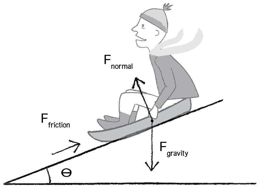
In Chapter 2, we learned how a force (such as the force of gravity in Figure 3.11) causes an object to accelerate. F = M * A or A = F / M. In this case, however, the pendulum bob doesn’t simply fall to the ground because it is attached by an arm to the pivot point. And so, in order to determine its angular acceleration, we not only need to look at the force of gravity, but also the force at the angle of the pendulum’s arm (relative to a pendulum at rest with an angle of 0).

In the above case, since the pendulum’s arm is of fixed length, the only variable in the scenario is the angle. We are going to simulate the pendulum’s motion through the use of angular velocity and acceleration. The angular acceleration will be calculated using Newton’s second law with a little trigonometry twist.

Let’s zoom in on the right triangle from the pendulum diagram.

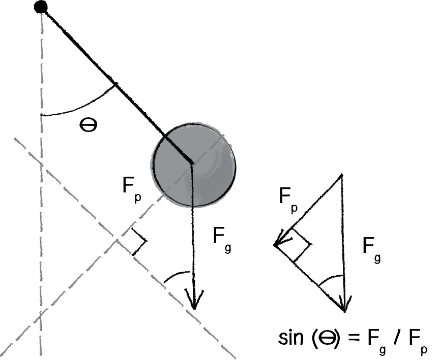
Figure 3.12

We can see that the force of the pendulum (F_p) should point perpendicular to the arm of the pendulum in the direction that the pendulum is swinging. After all, if there were no arm, the bob would just fall straight down. It’s the tension force of the arm that keeps the bob accelerating towards the pendulum’s rest state. Since the force of gravity (F_p) points downward, by making a right triangle out of these two vectors, we’ve accomplished something quite magnificent. We’ve made the force of gravity the hypotenuse of a right triangle and separated the vector into two components, one of which represents the force of the pendulum. Since sine equals opposite over hypotenuse, we have:

sine(θ) = F_p / F_g

Therefore:

F_p = F_g * sine(θ)

Lest we forget, we’ve been doing all of this with a single question in mind: What is the angular acceleration of the pendulum? Once we have the angular acceleration, we’ll be able to apply our rules of motion to find the new angle for the pendulum.

angular velocity = angular velocity + angular acceleration
angle = angle + angular velocity

The good news is that with Newton’s second law, we know that there is a relationship between force and acceleration, namely F = M * A, or A = F / M. So if the force of the pendulum is equal to the force of gravity times sine of the angle, then:

pendulum angular acceleration = acceleration due to gravity * sine (θ)

This is a good time to remind ourselves that we’re Processing programmers and not physicists. Yes, we know that the acceleration due to gravity on earth is 9.8 meters per second squared. But this number isn’t relevant to us. What we have here is just an arbitrary constant (we’ll call it gravity), one that we can use to scale the acceleration to something that feels right.

angular acceleration = gravity * sine(θ)

Amazing. After all that, the formula is so simple. You might be wondering, why bother going through the derivation at all? I mean, learning is great and all, but we could have easily just said, "Hey, the angular acceleration of a pendulum is some constant times the sine of the angle." This is just another moment in which we remind ourselves that the purpose of the book is not to learn how pendulums swing or gravity works. The point is to think creatively about how things can move about the screen in a computationally based graphics system. The pendulum is just a case study. If you can understand the approach to programming a pendulum, then however you choose to design your onscreen world, you can apply the same techniques.

Of course, we’re not finished yet. We may be happy with our simple, elegant formula, but we still have to apply it in code. This is most definitely a good time to practice our object-oriented programming skills and create a Pendulum class. Let’s think about all the properties we’ve encountered in our pendulum discussion that the class will need:

class Pendulum  {
 

  float r;

  float angle;

  float aVelocity;

  float aAcceleration;

We’ll also need to write a function update() to update the pendulum’s angle according to our formula…

  void update() {

    float gravity = 0.4;

    aAcceleration = -1 * gravity * sin(angle);

    aVelocity += aAcceleration;

    angle += aVelocity;
  }

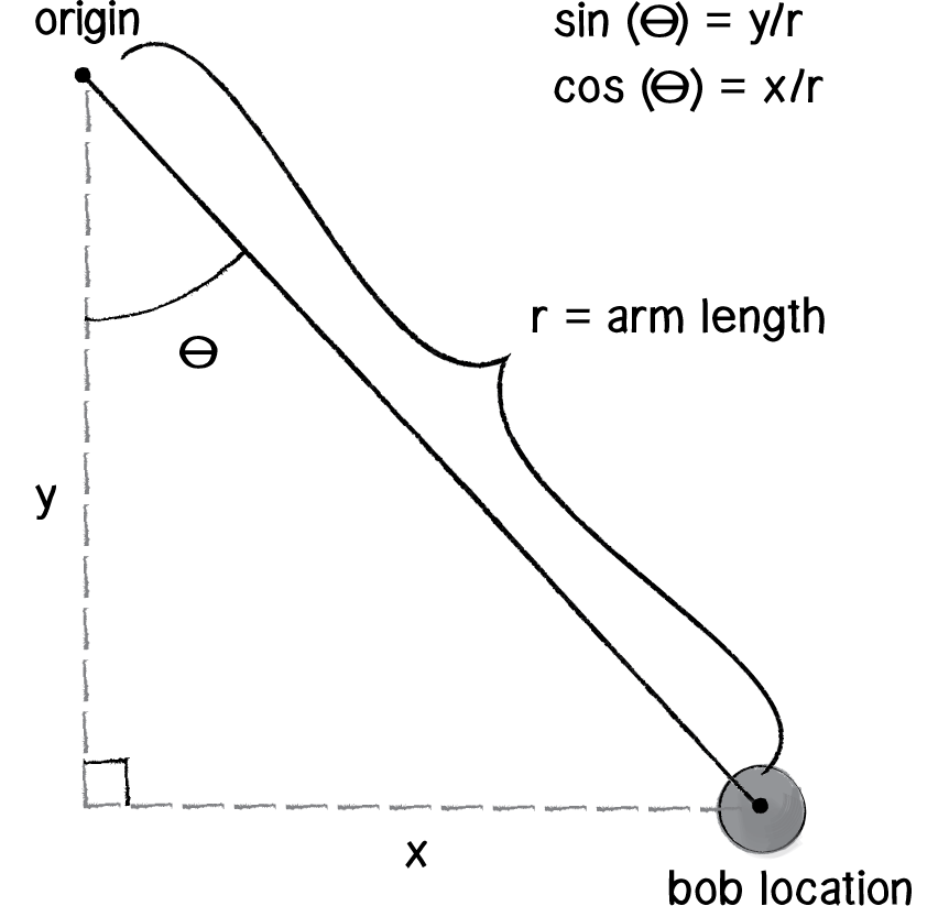
Figure 3.13

…as well as a function display() to draw the pendulum in the window. This begs the question: “Um, where do we draw the pendulum?” We know the angle and the arm length, but how do we know the x,y (Cartesian!) coordinates for both the pendulum’s pivot point (let’s call it origin) and bob location (let’s call it location)? This may be getting a little tiring, but the answer, yet again, is trigonometry.

The origin is just something we make up, as is the arm length. Let’s say:

PVector origin = new PVector(100,10);
float r = 125;

We’ve got the current angle stored in our variable angle. So relative to the origin, the pendulum’s location is a polar coordinate: (r,angle). And we need it to be Cartesian. Luckily for us, we just spent some time (section 3.5) deriving the formula for converting from polar to Cartesian. And so:

PVector location = new PVector(r*sin(angle),r*cos(angle));

Since the location is relative to wherever the origin happens to be, we can just add origin to the location PVector:

location.add(origin);

And all that remains is the little matter of drawing a line and ellipse (you should be more creative, of course).

stroke(0);
fill(175);
line(origin.x,origin.y,location.x,location.y);
ellipse(location.x,location.y,16,16);

Before we put everything together, there’s one last little detail I neglected to mention. Let’s think about the pendulum arm for a moment. Is it a metal rod? A string? A rubber band? How is it attached to the pivot point? How long is it? What is its mass? Is it a windy day? There are a lot of questions that we could continue to ask that would affect the simulation. We’re living, of course, in a fantasy world, one where the pendulum’s arm is some idealized rod that never bends and the mass of the bob is concentrated in a single, infinitesimally small point. Nevertheless, even though we don’t want to worry ourselves with all of the questions, we should add one more variable to our calculation of angular acceleration. To keep things simple, in our derivation of the pendulum’s acceleration, we assumed that the length of the pendulum’s arm is 1. In fact, the length of the pendulum’s arm affects the acceleration greatly: the longer the arm, the slower the acceleration. To simulate a pendulum more accurately, we divide by that length, in this case r. For a more involved explanation, visit The Simple Pendulum website.

aAcceleration = (-1 * G * sin(angle)) / r;

Finally, a real-world pendulum is going to experience some amount of friction (at the pivot point) and air resistance. With our code as is, the pendulum would swing forever, so to make it more realistic we can use a “damping” trick. I say trick because rather than model the resistance forces with some degree of accuracy (as we did in Chapter 2), we can achieve a similar result by simply reducing the angular velocity during each cycle. The following code reduces the velocity by 1% (or multiplies it by 99%) during each frame of animation:

aVelocity *= 0.99;

Putting everything together, we have the following example (with the pendulum beginning at a 45-degree angle).

Example 3.10: Swinging pendulum

Pendulum p;
 
void setup() {
  size(640,360);

  p = new Pendulum(new PVector(width/2,10),125);
}
 
void draw() {
  background(255);
  p.go();
}
 
class Pendulum  {

  PVector location;    // Location of bob
  PVector origin;      // Location of arm origin
  float r;             // Length of arm
  float angle;         // Pendulum arm angle
  float aVelocity;     // Angle velocity
  float aAcceleration; // Angle acceleration
  float damping;       // Arbitrary damping amount

 
  Pendulum(PVector origin_, float r_) {
    origin = origin_.get();
    location = new PVector();
    r = r_;
    angle = PI/4;
 
    aVelocity = 0.0;
    aAcceleration = 0.0;

    damping = 0.995;
  }
 
  void go() {
    update();
    display();
  }
 
  void update() {
    float gravity = 0.4;

    aAcceleration = (-1 * gravity / r) * sin(angle);
 

    aVelocity += aAcceleration;
    angle += aVelocity;

    aVelocity *= damping;
  }
 
  void display() {

    location.set(r*sin(angle),r*cos(angle),0);
    location.add(origin);
 
    stroke(0);

    line(origin.x,origin.y,location.x,location.y);
    fill(175);

    ellipse(location.x,location.y,16,16);
  }
}

(Note that the version of the example posted on the website has additional code to allow the user to grab the pendulum and swing it with the mouse.)

Exercise 3.13

Using trigonometry, what is the magnitude of the normal force in the illustration on the right (the force perpendicular to the incline on which the sled rests)? Note that, as indicated, the “normal” force is a component of the force of gravity.

3.10 Spring Forces

In section 3.6, we looked at modeling simple harmonic motion by mapping the sine wave to a pixel range. Exercise 3.6 asked you to use this technique to create a simulation of a bob hanging from a spring. While using the sin() function is a quick-and-dirty, one-line-of-code way of getting something up and running, it won’t do if what we really want is to have a bob hanging from a spring in a two-dimensional space that responds to other forces in the environment (wind, gravity, etc.) To accomplish a simulation like this (one that is identical to the pendulum example, only now the arm is a springy connection), we need to model the forces of a spring using PVector.

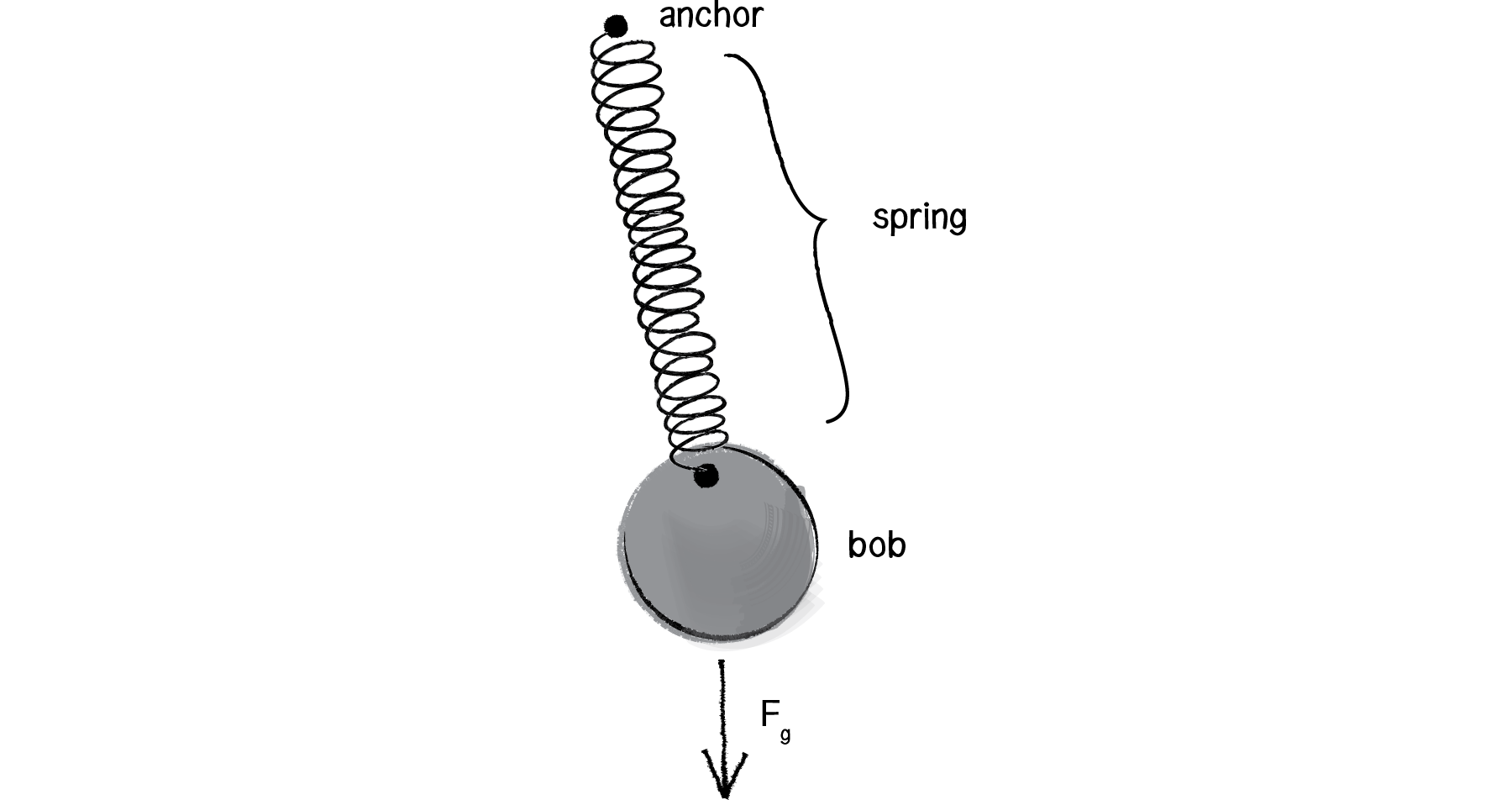
Figure 3.14

The force of a spring is calculated according to Hooke’s law, named for Robert Hooke, a British physicist who developed the formula in 1660. Hooke originally stated the law in Latin: "Ut tensio, sic vis," or “As the extension, so the force.” Let’s think of it this way:

The force of the spring is directly proportional to the extension of the spring.

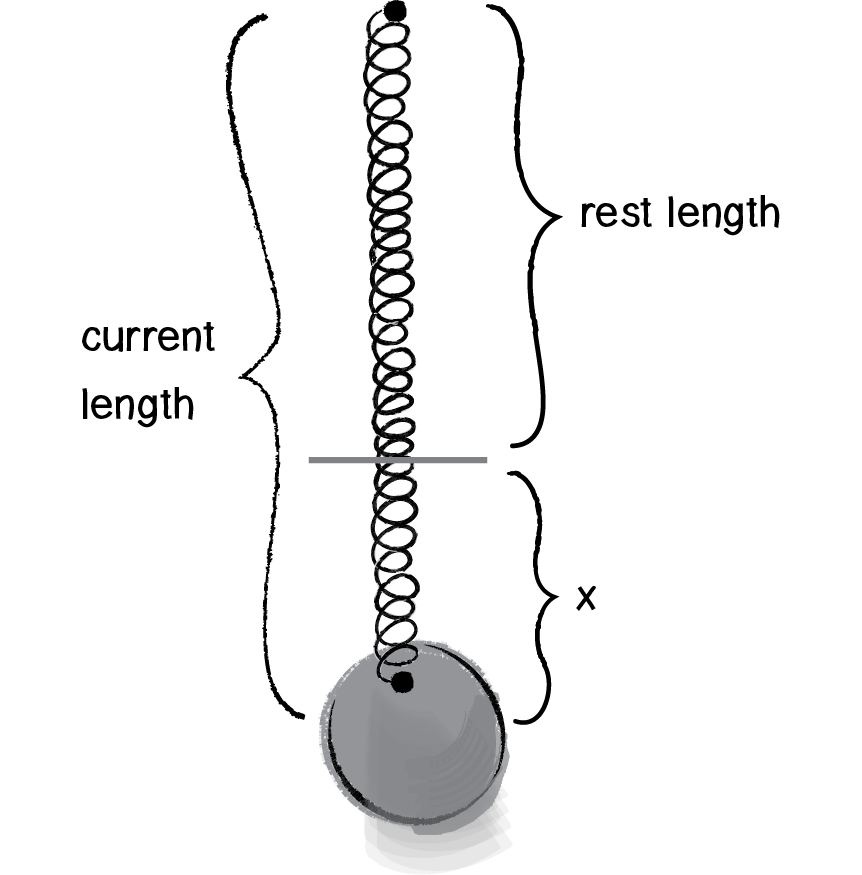
Figure 3.15: x = current length - rest length

In other words, if you pull on the bob a lot, the force will be strong; if you pull on the bob a little, the force will be weak. Mathematically, the law is stated as follows:

F_spring = - k * x

Now remember, force is a vector, so we need to calculate both magnitude and direction. Let’s look at one more diagram of the spring and label all the givens we might have in a Processing sketch.

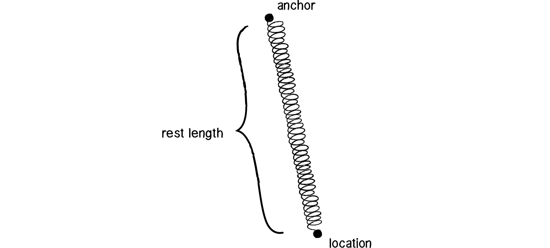
Figure 3.16

Let’s establish the following three variables as shown in Figure 3.16.

PVector anchor;
PVector location;
float restLength;

First, let’s use Hooke’s law to calculate the magnitude of the force. We need to know k and x. k is easy; it’s just a constant, so let’s make something up.

float k = 0.1;

x is perhaps a bit more difficult. We need to know the “difference between the current length and the rest length.” The rest length is defined as the variable restLength. What’s the current length? The distance between the anchor and the bob. And how can we calculate that distance? How about the magnitude of a vector that points from the anchor to the bob? (Note that this is exactly the same process we employed when calculating distance in Example 2.9: gravitational attraction.)

PVector dir = PVector.sub(bob,anchor);
float currentLength = dir.mag();
float x = restLength - currentLength;

Now that we’ve sorted out the elements necessary for the magnitude of the force (-1 * k * x), we need to figure out the direction, a unit vector pointing in the direction of the force. The good news is that we already have this vector. Right? Just a moment ago we thought to ourselves: “How we can calculate that distance? How about the magnitude of a vector that points from the anchor to the bob?” Well, that is the direction of the force!

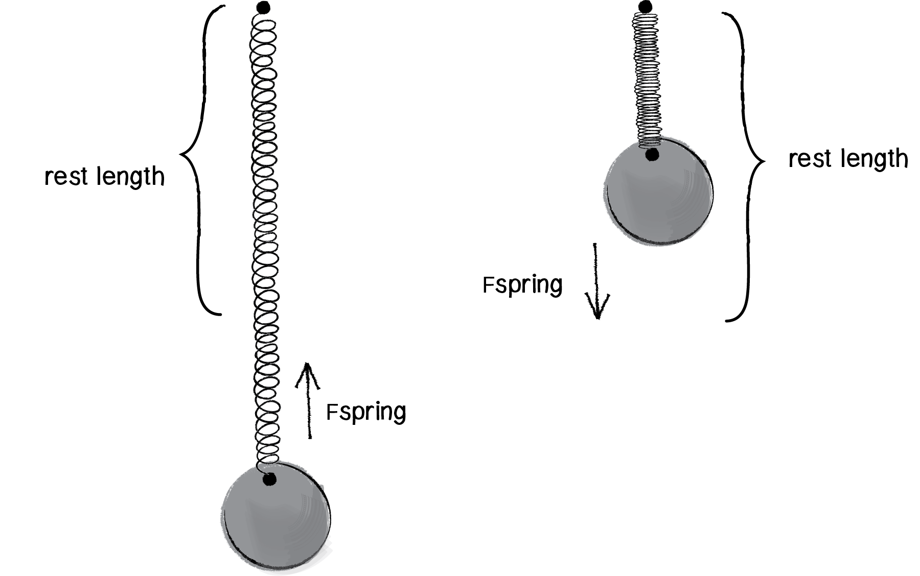
Figure 3.17

In Figure 3.17, we can see that if we stretch the spring beyond its rest length, there should be a force pulling it back towards the anchor. And if it shrinks below its rest length, the force should push it away from the anchor. This reversal of direction is accounted for in the formula with the -1. And so all we need to do is normalize the PVector we used for the distance calculation! Let’s take a look at the code and rename that PVector variable as “force.”

float k = 0.1;
PVector force = PVector.sub(bob,anchor);
float currentLength = dir.mag();
float x = restLength - currentLength;
 

force.normalize();
 

force.mult(-1 * k * x);

Now that we have the algorithm worked out for computing the spring force vector, the question remains: what object-oriented programming structure should we use? This, again, is one of those situations in which there is no “correct” answer. There are several possibilities; which one we choose depends on the program’s goals and one’s own personal coding style. Still, since we’ve been working all along with a Mover class, let’s keep going with this same framework. Let’s think of our Mover class as the spring’s “bob.” The bob needs location, velocity, and acceleration vectors to move about the screen. Perfect—we’ve got that already! And perhaps the bob experiences a gravity force via the applyForce() function. Just one more step—we need to apply the spring force:

Bob bob;
 
void setup() {
  bob = new Bob();
}
 
void draw()  {

  PVector gravity = new PVector(0,1);
  bob.applyForce(gravity);

  PVector springForce = _______________????
  bob.applyForce(springForce);

  bob.update();
  bob.display();
}

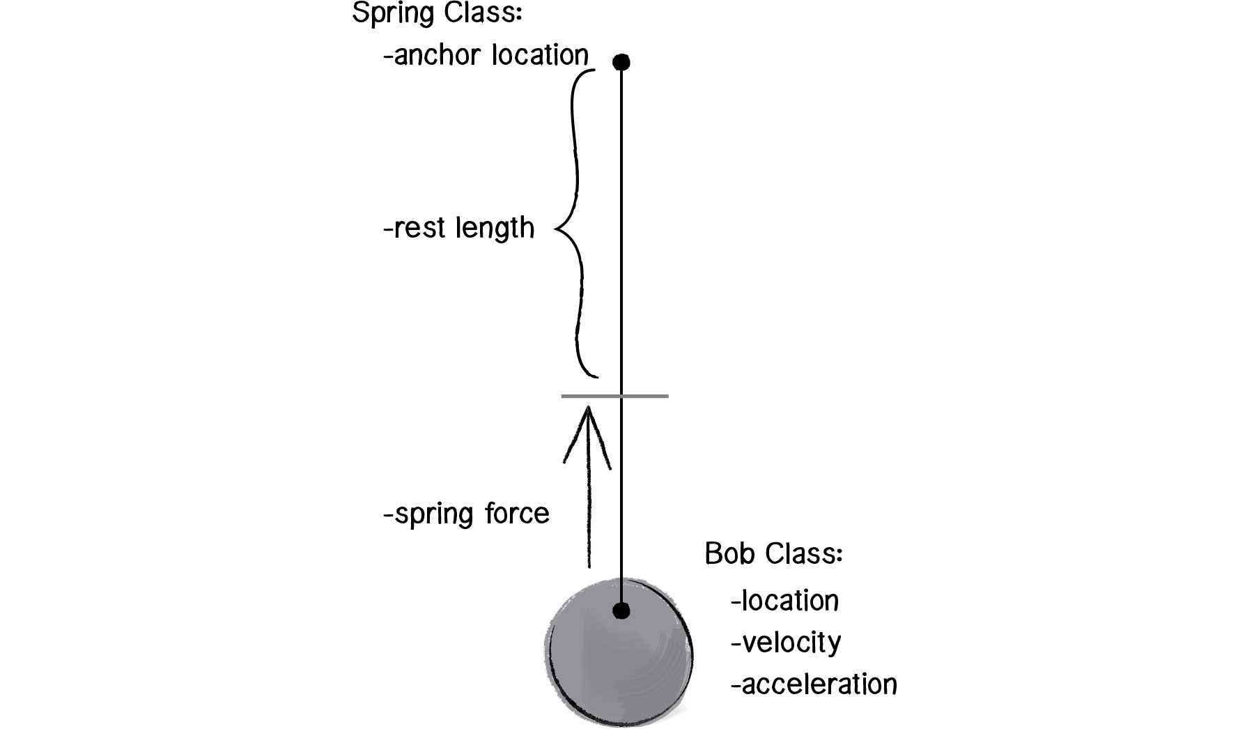
Figure 3.18

One option would be to write out all of the spring force code in the main draw() loop. But thinking ahead to when you might have multiple bobs and multiple spring connections, it makes a good deal of sense to write an additional class, a Spring class. As shown in Figure 3.18, the Bob class keeps track of the movements of the bob; the Spring class keeps track of the spring’s anchor and its rest length and calculates the spring force on the bob.

This allows us to write a lovely main program as follows:

Bob bob;

Spring spring;
 
void setup() {
  bob = new Bob();
  spring = new Spring();
}
 
void draw()  {
  PVector gravity = new PVector(0,1);
  bob.applyForce(gravity);
 

  spring.connect(bob);
 
  bob.update();
  bob.display();
  spring.display();
}

You may notice here that this is quite similar to what we did in Example 2.6 with an attractor. There, we said something like:

  PVector force = attractor.attract(mover);
  mover.applyForce(force);

The analogous situation here with a spring would be:

  PVector force = spring.connect(bob);
  bob.applyForce(force);

Nevertheless, in this example all we said was:

  spring.connect(bob);

What gives? Why don’t we need to call applyForce() on the bob? The answer is, of course, that we do need to call applyForce() on the bob. Only instead of doing it in draw(), we’re just demonstrating that a perfectly reasonable (and sometimes preferable) alternative is to ask the connect() function to internally handle calling applyForce() on the bob.

  void connect(Bob b) {
    PVector force = some fancy calculations
 

    b.applyForce(force);
  }

Why do it one way with the Attractor class and another way with the Spring class? When we were first learning about forces, it was a bit clearer to show all the forces being applied in the main draw() loop, and hopefully this helped you learn about force accumulation. Now that we’re more comfortable with that, perhaps it’s simpler to embed some of the details inside the objects themselves.

Let’s take a look at the rest of the elements in the Spring class.

Example 3.11: A Spring connection

class Spring {
 

  PVector anchor;
 

  float len;
  float k = 0.1;
 

  Spring(float x, float y, int l) {
    anchor = new PVector(x,y);
    len = l;
  }

  void connect(Bob b) {
 

    PVector force =
      PVector.sub(b.location,anchor);

    float d = force.mag();

    float stretch = d - len;
 

    force.normalize();
    force.mult(-1 * k * stretch);

    b.applyForce(force);
  }
 

  void display() {
    fill(100);
    rectMode(CENTER);
    rect(anchor.x,anchor.y,10,10);
  }

  void displayLine(Bob b) {
    stroke(255);
    line(b.location.x,b.location.y,anchor.x,anchor.y);
  }

 
}

The full code for this example is included on the book website, and the Web version also incorporates two additional features: (1) the Bob class includes functions for mouse interactivity so that the bob can be dragged around the window, and (2) the Spring object includes a function to constrain the connection’s length between a minimum and a maximum.

void constrainLength(Bob b, float minlen, float maxlen) {

  PVector dir = PVector.sub(______,______);
  float d = dir.mag();
 

  if (d < minlen) {
    dir.normalize();
    dir.mult(________);

    b.location = PVector.add(______,______);
    b.velocity.mult(0);

  } else if (____________) {
    dir.normalize();
    dir.mult(_________);

    b.location = PVector.add(______,______);
    b.velocity.mult(0);
  }
}