Chapter 8. Fractals
“Pathological monsters! cried the terrified mathematician
Every one of them a splinter in my eye
I hate the Peano Space and the Koch Curve
I fear the Cantor Ternary Set
The Sierpinski Gasket makes me wanna cry
And a million miles away a butterfly flapped its wings
On a cold November day a man named Benoit Mandelbrot was born”
— Jonathan Coulton, lyrics from “Mandelbrot Set”
Once upon a time, I took a course in high school called “Geometry.” Perhaps you did too. You learned about shapes in one dimension, two dimensions, and maybe even three. What is the circumference of a circle? The area of a rectangle? The distance between a point and a line? Come to think of it, we’ve been studying geometry all along in this book, using vectors to describe the motion of bodies in Cartesian space. This sort of geometry is generally referred to as Euclidean geometry, after the Greek mathematician Euclid.
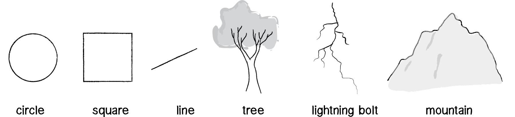
Figure 8.1
For us nature coders, we have to ask the question: Can we describe our world with Euclidean geometry? The LCD screen I’m staring at right now sure looks like a rectangle. And the plum I ate this morning is circular. But what if I were to look further, and consider the trees that line the street, the leaves that hang off those trees, the lightning from last night’s thunderstorm, the cauliflower I ate for dinner, the blood vessels in my body, and the mountains and coastlines that cover land beyond New York City? Most of the stuff you find in nature cannot be described by the idealized geometrical forms of Euclidean geometry. So if we want to start building computational designs with patterns beyond the simple shapes ellipse(), rect(), and line(), it’s time for us to learn about the concepts behind and techniques for simulating the geometry of nature: fractals.
8.1 What Is a Fractal?
The term fractal (from the Latin fractus, meaning “broken”) was coined by the mathematician Benoit Mandelbrot in 1975. In his seminal work “The Fractal Geometry of Nature,” he defines a fractal as “a rough or fragmented geometric shape that can be split into parts, each of which is (at least approximately) a reduced-size copy of the whole.”

Figure 8.2: One of the most well-known and recognizable fractal patterns is named for Benoit Mandelbrot himself. Generating the Mandelbrot set involves testing the properties of complex numbers after they are passed through an iterative function. Do they tend to infinity? Do they stay bounded? While a fascinating mathematical discussion, this “escape-time” algorithm is a less practical method for generating fractals than the recursive techniques we’ll examine in this chapter. However, an example for generating the Mandelbrot set is included in the code examples.
Let’s illustrate this definition with two simple examples. First, let’s think about a tree branching structure (for which we’ll write the code later):
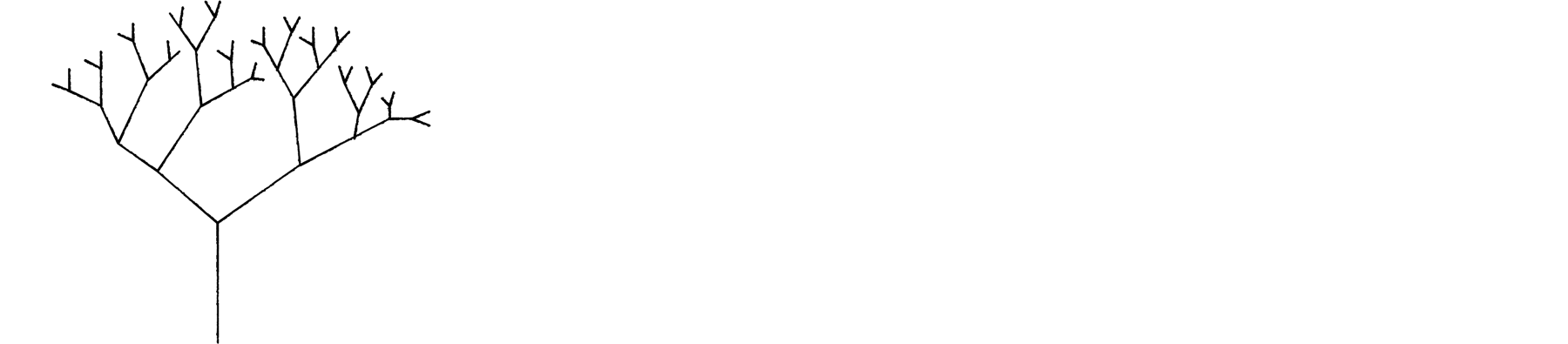
Figure 8.3
Notice how the tree in Figure 8.3 has a single root with two branches connected at its end. Each one of those branches has two branches at its end and those branches have two branches and so on and so forth. What if we were to pluck one branch from the tree and examine it on its own?
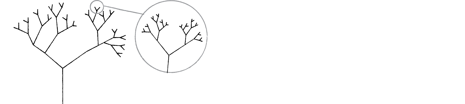
Figure 8.4
Looking closely at a given section of the tree, we find that the shape of this branch resembles the tree itself. This is known as self-similarity; as Mandelbrot stated, each part is a “reduced-size copy of the whole.”
The above tree is perfectly symmetrical and the parts are, in fact, exact replicas of the whole. However, fractals do not have to be perfectly self-similar. Let’s take a look at a graph of the stock market (adapted from actual Apple stock data).
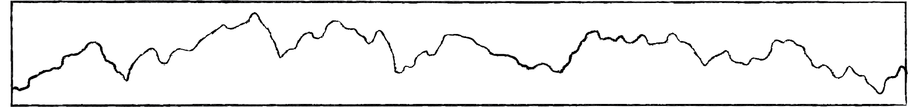
Figure 8.5: Graph A
And one more.
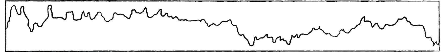
Figure 8.6: Graph B
In these graphs, the x-axis is time and the y-axis is the stock’s value. It’s not an accident that I omitted the labels, however. Graphs of stock market data are examples of fractals because they look the same at any scale. Are these graphs of the stock over one year? One day? One hour? There’s no way for you to know without a label. (Incidentally, graph A shows six months’ worth of data and graph B zooms into a tiny part of graph A, showing six hours.)
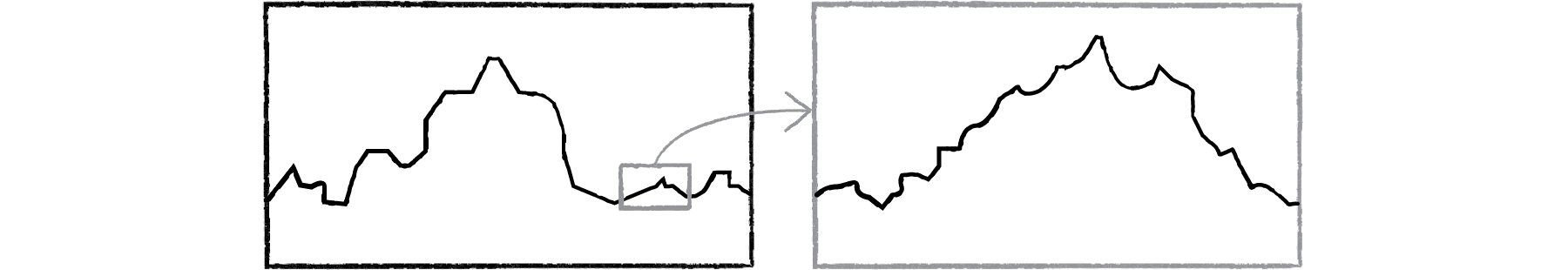
Figure 8.7
This is an example of a stochastic fractal, meaning that it is built out of probabilities and randomness. Unlike the deterministic tree-branching structure, it is statistically self-similar. As we go through the examples in this chapter, we will look at both deterministic and stochastic techniques for generating fractal patterns.
While self-similarity is a key trait of fractals, it’s important to realize that self-similarity alone does not make a fractal. After all, a line is self-similar. A line looks the same at any scale, and can be thought of as comprising lots of little lines. But it’s not a fractal. Fractals are characterized by having a fine structure at small scales (keep zooming into the stock market graph and you’ll continue to find fluctuations) and cannot be described with Euclidean geometry. If you can say “It’s a line!” then it’s not a fractal.
Another fundamental component of fractal geometry is recursion. Fractals all have a recursive definition. We’ll start with recursion before developing techniques and code examples for building fractal patterns in Processing.
8.2 Recursion
Let’s begin our discussion of recursion by examining the first appearance of fractals in modern mathematics. In 1883, German mathematician George Cantor developed simple rules to generate an infinite set:

Figure 8.8: The Cantor set
There is a feedback loop at work here. Take a single line and break it into two. Then return to those two lines and apply the same rule, breaking each line into two, and now we’re left with four. Then return to those four lines and apply the rule. Now you’ve got eight. This process is known as recursion: the repeated application of a rule to successive results. Cantor was interested in what happens when you apply these rules an infinite number of times. We, however, are working in a finite pixel space and can mostly ignore the questions and paradoxes that arise from infinite recursion. We will instead construct our code in such a way that we do not apply the rules forever (which would cause our program to freeze).
Before we implement the Cantor set, let’s take a look at what it means to have recursion in code. Here’s something we’re used to doing all the time—calling a function inside another function.
  background(0);
}
What would happen if we called the function we are defining within the function itself? Can someFunction() call someFunction()?
void someFunction() {
  someFunction();
}
In fact, this is not only allowed, but it’s quite common (and essential to how we will implement the Cantor set). Functions that call themselves are recursive and good for solving certain problems. For example, certain mathematical calculations are implemented recursively; the most common example is factorial.
The factorial of any number n, usually written as n!, is defined as:
n! = n * n – 1 * . . . . * 3 * 2 * 1
0! = 1
Here we’ll write a function in Processing that uses a for loop to calculate factorial:
int factorial(int n) {
  int f = 1;
  for (int i = 0; i < n; i++) {
    f = f * (i+1);
  }
  return f;
}
Upon close examination, you’ll notice something interesting about how factorial works. Let’s look at 4! and 3!
4! = 4 * 3 * 2 * 1
3! = 3 * 2 * 1
therefore. . .
4! = 4 * 3!
In more general terms, for any positive integer n:
n! = n * (n-1)!
1! = 1
Written out:
The factorial of n is defined as n times the factorial of n-1.
The definition of factorial includes factorial?! It’s kind of like defining “tired" as “the feeling you get when you are tired.” This concept of self-reference in functions is an example of recursion. And we can use it to write a factorial function that calls itself.
int factorial(int n) {
  if (n == 1) {
    return 1;
  } else {
    return n * factorial(n-1);
  }
}
It may look crazy, but it works. Here are the steps that happen when factorial(4) is called.
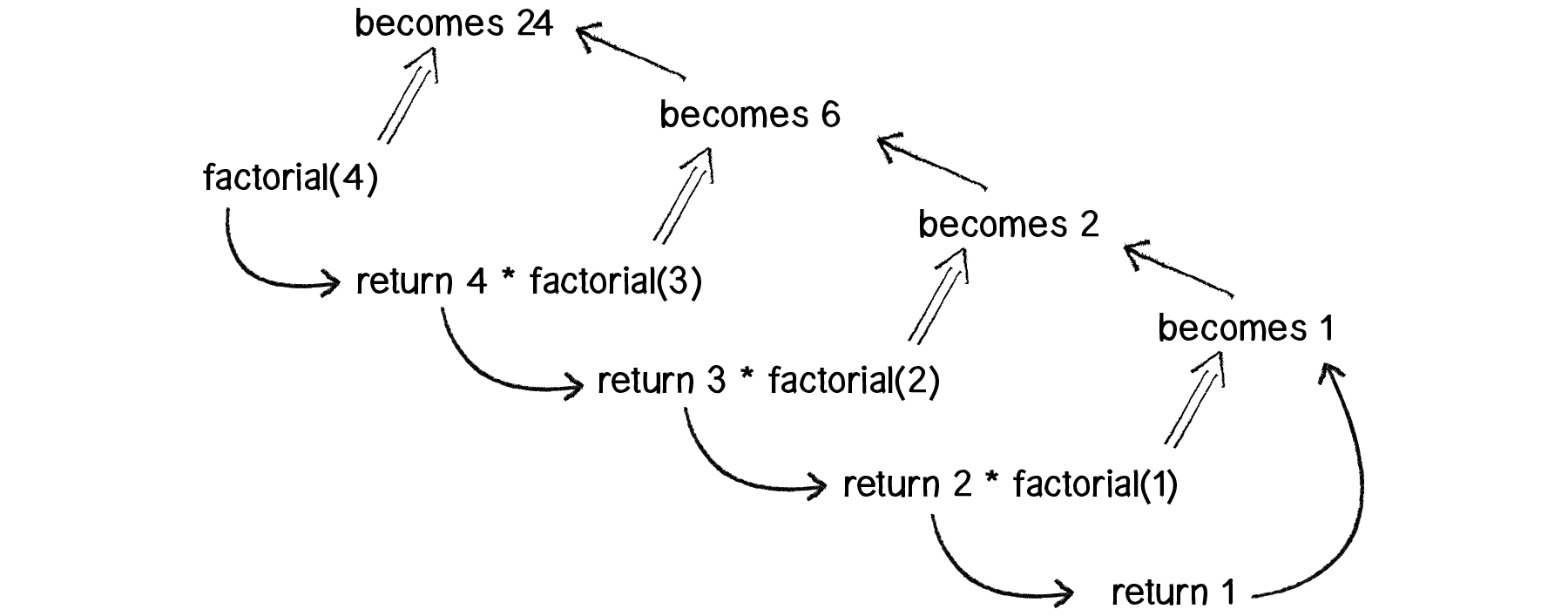
Figure 8.9
We can apply the same principle to graphics with interesting results, as we will see in many examples throughout this chapter. Take a look at this recursive function.
Example 8.1: Recursive Circles I
void drawCircle(int x, int y, float radius) {
  ellipse(x, y, radius, radius);
  if(radius > 2) {
    radius *= 0.75f;
    drawCircle(x, y, radius);
  }
}
drawCircle() draws an ellipse based on a set of parameters that it receives as arguments. It then calls itself with those same parameters, adjusting them slightly. The result is a series of circles, each of which is drawn inside the previous circle.
Notice that the above function only recursively calls itself if the radius is greater than 2. This is a crucial point. As with iteration, all recursive functions must have an exit condition! You likely are already aware that all for and while loops must include a boolean expression that eventually evaluates to false, thus exiting the loop. Without one, the program would crash, caught inside of an infinite loop. The same can be said about recursion. If a recursive function calls itself forever and ever, you’ll be most likely be treated to a nice frozen screen.
This circles example is rather trivial; it could easily be achieved through simple iteration. However, for scenarios in which a function calls itself more than once, recursion becomes wonderfully elegant.
Let’s make drawCircle() a bit more complex. For every circle displayed, draw a circle half its size to the left and right of that circle.
void setup() {
  size(640,360);
}

void draw() {
  background(255);
  drawCircle(width/2,height/2,200);
}

void drawCircle(float x, float y, float radius) {
  stroke(0);
  noFill();
  ellipse(x, y, radius, radius);
  if(radius > 2) {
    drawCircle(x + radius/2, y, radius/2);
    drawCircle(x - radius/2, y, radius/2);
  }
}
With just a little more code, we could also add a circle above and below each circle.
Example 8.3: Recursion four times
void drawCircle(float x, float y, float radius) {
  ellipse(x, y, radius, radius);
  if(radius > 8) {
    drawCircle(x + radius/2, y, radius/2);
    drawCircle(x - radius/2, y, radius/2);
    drawCircle(x, y + radius/2, radius/2);
    drawCircle(x, y - radius/2, radius/2);
  }
}
Try reproducing this sketch with iteration instead of recursion—I dare you!
8.3 The Cantor Set with a Recursive Function
Now we’re ready to visualize the Cantor set in Processing using a recursive function. Where do we begin? Well, we know that the Cantor set begins with a line. So let’s start there and write a function that draws a line.
void cantor(float x, float y, float len) {
  line(x,y,x+len,y);
}
The above cantor() function draws a line that starts at pixel coordinate (x,y) with a length of len. (The line is drawn horizontally here, but this is an arbitrary decision.) So if we called that function, saying:
cantor(10, 20, width-20);we’d get the following:

Figure 8.10
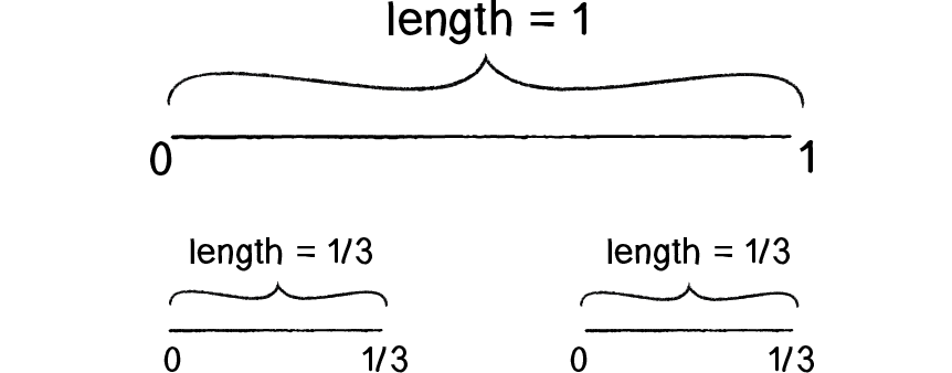
Figure 8.11
Now, the Cantor rule tells us to erase the middle third of that line, which leaves us with two lines, one from the beginning of the line to the one-third mark, and one from the two-thirds mark to the end of the line.
We can now add two more lines of code to draw the second pair of lines, moving the y-location down a bunch of pixels so that we can see the result below the original line.
void cantor(float x, float y, float len) {
  line(x,y,x+len,y);

  y += 20;
line(x,y,x+len/3,y); line(x+len*2/3,y,x+len,y);
}

Figure 8.12
While this is a fine start, such a manual approach of calling line() for each line is not what we want. It will get unwieldy very quickly, as we’d need four, then eight, then sixteen calls to line(). Yes, a for loop is our usual way around such a problem, but give that a try and you’ll see that working out the math for each iteration quickly proves inordinately complicated. Here is where recursion comes and rescues us.
Take a look at where we draw that first line from the start to the one-third mark.
line(x,y,x+len/3,y);Instead of calling the line() function directly, we can simply call the cantor() function itself. After all, what does the cantor() function do? It draws a line at an (x,y) location with a given length! And so:
line(x,y,x+len/3,y); becomes -------> cantor(x,y,len/3);And for the second line:
line(x+len*2/3,y,x+len,y); becomes -------> cantor(x+len*2/3,y,len/3);Leaving us with:
void cantor(float x, float y, float len) {
  line(x,y,x+len,y);

  y += 20;

  cantor(x,y,len/3);
  cantor(x+len*2/3,y,len/3);
}
And since the cantor() function is called recursively, the same rule will be applied to the next lines and to the next and to the next as cantor() calls itself again and again! Now, don’t go and run this code yet. We’re missing that crucial element: an exit condition. We’ll want to make sure we stop at some point—for example, if the length of the line ever is less than 1 pixel.
void cantor(float x, float y, float len) { if (len >= 1) {
line(x,y,x+len,y);
y += 20;
cantor(x,y,len/3);
cantor(x+len*2/3,y,len/3);
}
}
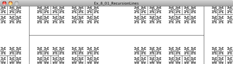
Exercise 8.1
Using drawCircle() and the Cantor set as models, generate your own pattern with recursion. Here is a screenshot of one that uses lines.
8.4 The Koch Curve and the ArrayList Technique
Writing a function that recursively calls itself is one technique for generating a fractal pattern on screen. However, what if you wanted the lines in the above Cantor set to exist as individual objects that could be moved independently? The recursive function is simple and elegant, but it does not allow you to do much besides simply generating the pattern itself. However, there is another way we can apply recursion in combination with an ArrayList that will allow us to not only generate a fractal pattern, but keep track of all its individual parts as objects.
To demonstrate this technique, let’s look at another famous fractal pattern, discovered in 1904 by Swedish mathematician Helge von Koch. Here are the rules. (Note that it starts the same way as the Cantor set, with a single line.)
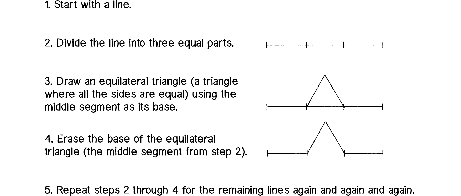
Figure 8.13
The result looks like:
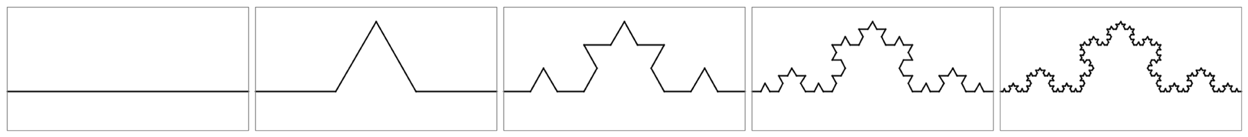
Figure 8.14
The “Monster” Curve
The Koch curve and other fractal patterns are often called “mathematical monsters.” This is due to an odd paradox that emerges when you apply the recursive definition an infinite number of times. If the length of the original starting line is one, the first iteration of the Koch curve will yield a line of length four-thirds (each segment is one-third the length of the starting line). Do it again and you get a length of sixteen-ninths. As you iterate towards infinity, the length of the Koch curve approaches infinity. Yet it fits in the tiny finite space provided right here on this paper (or screen)!
Since we are working in the Processing land of finite pixels, this theoretical paradox won’t be a factor for us. We’ll have to limit the number of times we recursively apply the Koch rules so that our program won’t run out of memory or crash.
We could proceed in the same manner as we did with the Cantor set, and write a recursive function that iteratively applies the Koch rules over and over. Nevertheless, we are going to tackle this problem in a different manner by treating each segment of the Koch curve as an individual object. This will open up some design possibilities. For example, if each segment is an object, we could allow each segment to move independently from its original location and participate in a physics simulation. In addition, we could use a random color, line thickness, etc. to display each segment differently.
In order to accomplish our goal of treating each segment as an individual object, we must first decide what this object should be in the first place. What data should it store? What functions should it have?
The Koch curve is a series of connected lines, and so we will think of each segment as a “KochLine.” Each KochLine object has a start point (“a”) and an end point (“b”). These points are PVector objects, and the line is drawn with Processing’s line() function.
class KochLine {
  PVector start;
  PVector end;
  KochLine(PVector a, PVector b) {
    start = a.get();
    end = b.get();
  }

  void display() {
    stroke(0);
    line(start.x, start.y, end.x, end.y);
  }
}
Now that we have our KochLine class, we can get started on the main program. We’ll need a data structure to keep track of what will eventually become many KochLine objects, and an ArrayList (see Chapter 4 for a review of ArrayLists) will do just fine.
ArrayList<KochLine> lines;In setup(), we’ll want to create the ArrayList and add the first line segment to it, a line that stretches from 0 to the width of the sketch.
void setup() {
  size(600, 300);
lines = new ArrayList<KochLine>();
PVector start = new PVector(0, 200); PVector end = new PVector(width, 200);
  lines.add(new KochLine(start, end));
}
Then in draw(), all KochLine objects (just one right now) can be displayed in a loop.
void draw() {
  background(255);
  for (KochLine l : lines) {
    l.display();
  }
}
This is our foundation. Let’s review what we have so far:
KochLine class: A class to keep track of a line from point A to B.
ArrayList: A list of all KochLine objects.
With the above elements, how and where do we apply Koch rules and principles of recursion?
Remember the Game of Life cellular automata? In that simulation, we always kept track of two generations: current and next. When we were finished computing the next generation, next became current and we moved on to computing the new next generation. We are going to apply a similar technique here. We have an ArrayList that keeps track of the current set of KochLine objects (at the start of the program, there is only one). We will need a second ArrayList (let’s call it “next”) where we will place all the new KochLine objects that are generated from applying the Koch rules. For every KochLine object in the current ArrayList, four new KochLine objects are added to the next ArrayList. When we’re done, the next ArrayList becomes the current one.
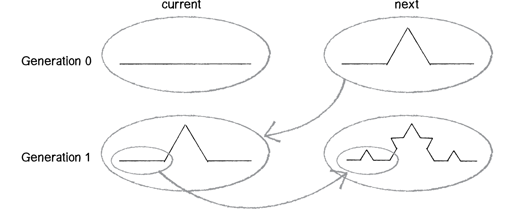
Figure 8.15
Here’s how the code will look:
void generate() { ArrayList next = new ArrayList<KochLine>();
for (KochLine l : lines) {
    next.add(new KochLine(???,???));
    next.add(new KochLine(???,???));
    next.add(new KochLine(???,???));
    next.add(new KochLine(???,???));
} lines = next;
}
By calling generate() over and over again (for example, each time the mouse is pressed), we recursively apply the Koch curve rules to the existing set of KochLine objects. Of course, the above omits the real “work” here, which is figuring out those rules. How do we break one line segment into four as described by the rules? While this can be accomplished with some simple arithmetic and trigonometry, since our KochLine object uses PVector, this is a nice opportunity for us to practice our vector math. Let’s establish how many points we need to compute for each KochLine object.
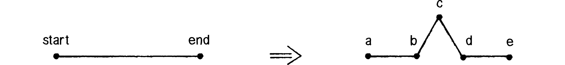
Figure 8.16
As you can see from the above figure, we need five points (a, b, c, d, and e) to generate the new KochLine objects and make the new line segments (ab, cb, cd, and de).
next.add(new KochLine(a,b));
next.add(new KochLine(b,c));
next.add(new KochLine(c,d));
next.add(new KochLine(d,e));
Where do we get these points? Since we have a KochLine object, why not ask the KochLine object to compute all these points for us?
void generate() {
ArrayList next = new ArrayList<KochLine>();
for (KochLine l : lines) {
PVector a = l.kochA();
PVector b = l.kochB();
PVector c = l.kochC();
PVector d = l.kochD();
PVector e = l.kochE();
next.add(new KochLine(a, b));
next.add(new KochLine(b, c));
next.add(new KochLine(c, d));
next.add(new KochLine(d, e));
}
  lines = next;
}
Now we just need to write five new functions in the KochLine class, each one returning a PVector according to Figure 8.16 above. Let’s knock off kochA() and kochE() first, which are simply the start and end points of the original line.
PVector kochA() { return start.get();
}
PVector kochE() {
return end.get();
}
Now let’s move on to points B and D. B is one-third of the way along the line segment and D is two-thirds. Here we can make a PVector that points from start to end and shrink it to one-third the length for B and two-thirds the length for D to find these points.
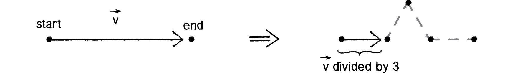
Figure 8.17
PVector kochB() { PVector v = PVector.sub(end, start); v.div(3); v.add(start);
return v;
}
PVector kochD() {
PVector v = PVector.sub(end, start);
    v.mult(2/3.0);
    v.add(start);
    return v;
  }
The last point, C, is the most difficult one to find. However, if you recall that the angles of an equilateral triangle are all sixty degrees, this makes it a little bit easier. If we know how to find point B with a PVector one-third the length of the line, what if we were to rotate that same PVector sixty degrees and move along that vector from point B? We’d be at point C!
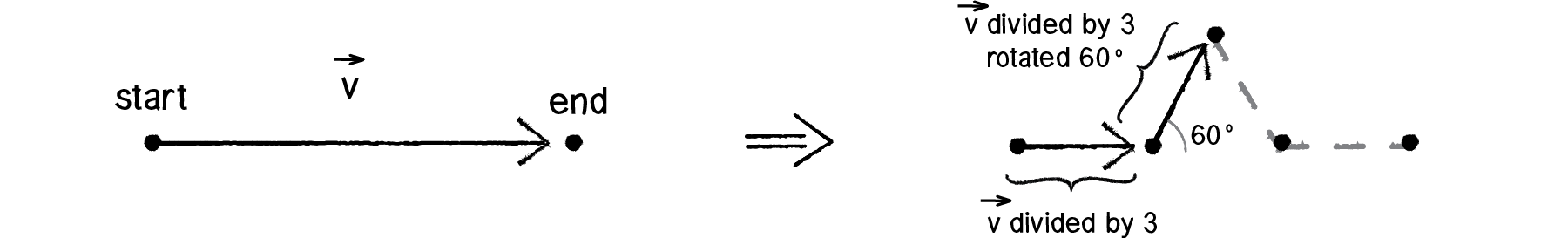
Figure 8.18
PVector kochC() { PVector a = start.get();
PVector v = PVector.sub(end, start);
    v.div(3);
    a.add(v);
v.rotate(-radians(60)); a.add(v);
return a;
}
Putting it all together, if we call generate() five times in setup(), we’ll see the following result.
ArrayList<KochLine> lines;

void setup() {
  size(600, 300);
  background(255);
  lines = new ArrayList<KochLine>();
  PVector start = new PVector(0, 200);
  PVector end   = new PVector(width, 200);
  lines.add(new KochLine(start, end));
  for (int i = 0; i < 5; i++) {
    generate();
  }
}
Exercise 8.2
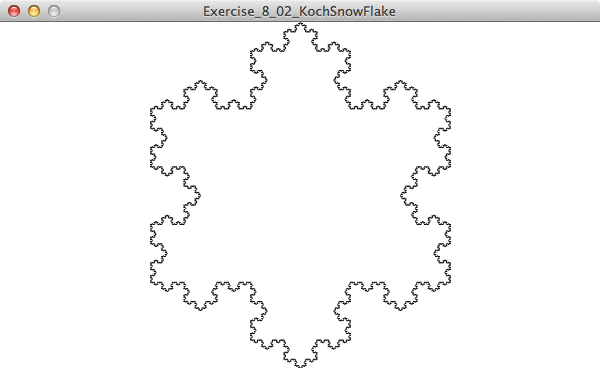
Draw the Koch snowflake (or some other variation of the Koch curve).

Exercise 8.3
Try animating the Koch curve. For example, can you draw it from left to right? Can you vary the visual design of the line segments? Can you move the line segments using techniques from earlier chapters? What if each line segment were made into a spring (toxiclibs) or joint (Box2D)?
Exercise 8.4
Rewrite the Cantor set example using objects and an ArrayList.
Exercise 8.5
Draw the Sierpiński triangle (as seen in Wolfram elementary CA) using recursion.

8.5 Trees
The fractals we have examined in this chapter so far are deterministic, meaning they have no randomness and will always produce the identical outcome each time they are run. They are excellent demonstrations of classic fractals and the programming techniques behind drawing them, but are too precise to feel natural. In this next part of the chapter, I want to examine some techniques behind generating a stochastic (or non-deterministic) fractal. The example we’ll use is a branching tree. Let’s first walk through the steps to create a deterministic version. Here are our production rules:
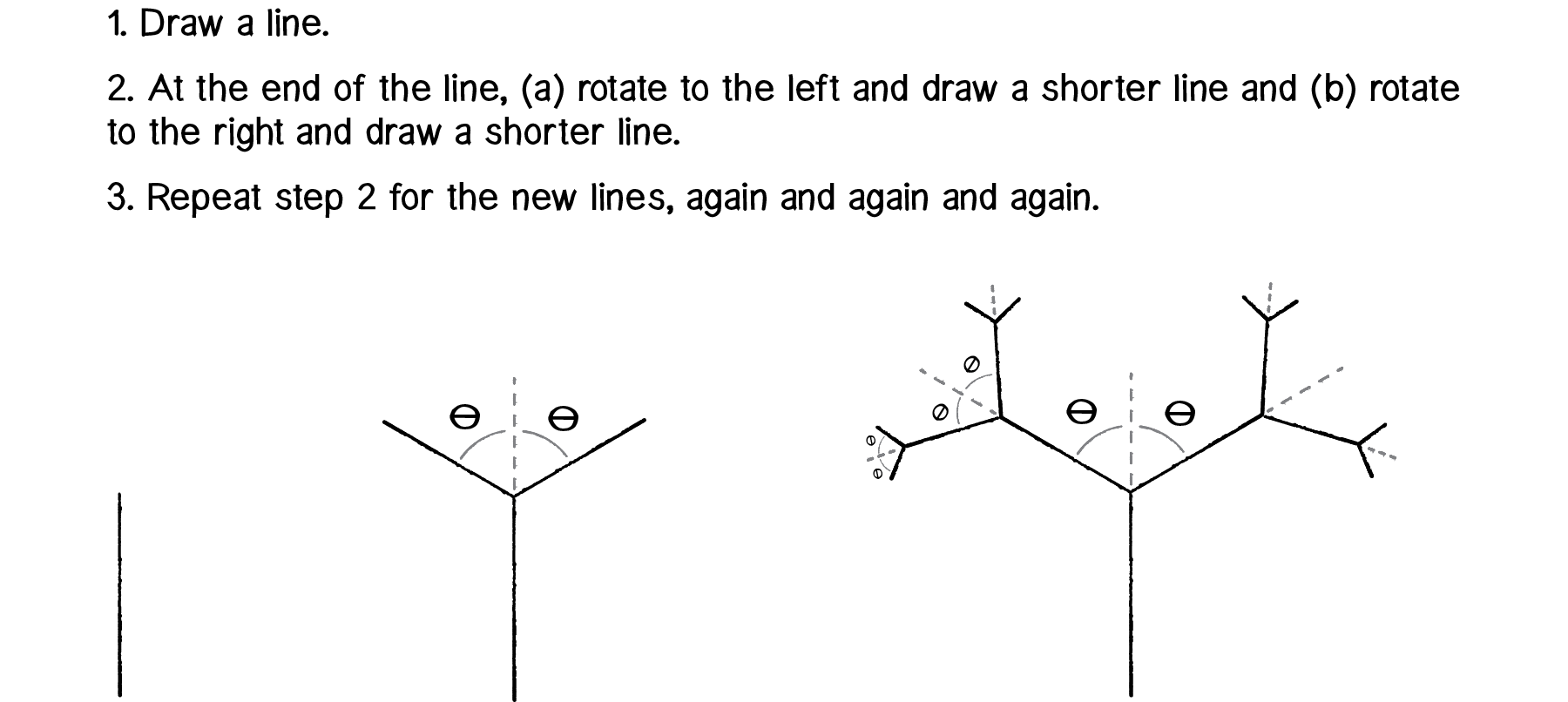
Figure 8.19
Again, we have a nice fractal with a recursive definition: A branch is a line with two branches connected to it.
The part that is a bit more difficult than our previous fractals lies in the use of the word rotate in the fractal’s rules. Each new branch must rotate relative to the previous branch, which is rotated relative to all its previous branches. Luckily for us, Processing has a mechanism to keep track of rotations for us—the transformation matrix. If you aren’t familiar with the functions pushMatrix() and popMatrix(), I suggest you read the online Processing tutorial 2D Transformations, which will cover the concepts you’ll need for this particular example.
Let’s begin by drawing a single branch, the trunk of the tree. Since we are going to involve the rotate() function, we’ll need to make sure we are continuously translating along the branches while we draw the tree. And since the root starts at the bottom of the window (see above), the first step requires translating to that spot:
translate(width/2,height);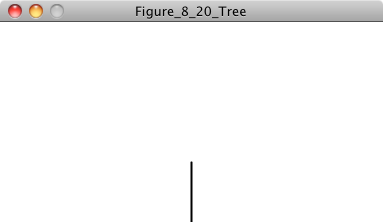
Figure 8.20
…followed by drawing a line upwards (Figure 8.20):
line(0,0,0,-100);Once we’ve finished the root, we just need to translate to the end and rotate in order to draw the next branch. (Eventually, we’re going to need to package up what we’re doing right now into a recursive function, but let’s sort out the steps first.)
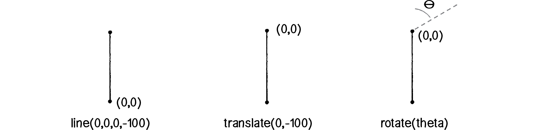
Figure 8.21
Remember, when we rotate in Processing, we are always rotating around the point of origin, so here the point of origin must always be translated to the end of our current branch.
translate(0,-100);
rotate(PI/6);
line(0,0,0,-100);
Now that we have a branch going to the right, we need one going to the left. We can use pushMatrix() to save the transformation state before we rotate, letting us call popMatrix() to restore that state and draw the branch to the left. Let’s look at all the code together.
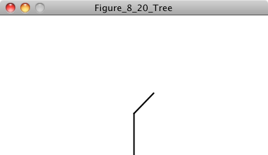
Figure 8.22
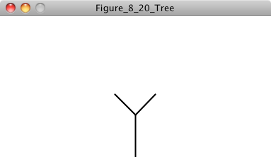
Figure 8.23
translate(width/2,height);line(0,0,0,-100);
translate(0,-100);
pushMatrix();
rotate(PI/6);
line(0,0,0,-100);
popMatrix();

rotate(-PI/6);
line(0,0,0,-100);If you think of each call to the function line() as a “branch,” you can see from the code above that we have implemented our definition of branching as a line that has two lines connected to its end. We could keep adding more and more calls to line() for more and more branches, but just as with the Cantor set and Koch curve, our code would become incredibly complicated and unwieldy. Instead, we can use the above logic as our foundation for writing a recursive function, replacing the direct calls to line() with our own function called branch(). Let’s take a look.
void branch() { line(0, 0, 0, -100); translate(0, -100);
pushMatrix();
  rotate(PI/6);
  branch();
  popMatrix();

  pushMatrix();
  rotate(-PI/6);
  branch();
  popMatrix();
}
Notice how in the above code we use pushMatrix() and popMatrix() around each subsequent call to branch(). This is one of those elegant code solutions that feels almost like magic. Each call to branch() takes a moment to remember the location of that particular branch. If you turn yourself into Processing for a moment and try to follow the recursive function with pencil and paper, you’ll notice that it draws all of the branches to the right first. When it gets to the end, popMatrix() will pop us back along all of the branches we’ve drawn and start sending branches out to the left.
Exercise 8.6

Emulate the Processing code in Example 8.6 and number the branches in the above diagram in the order that Processing would actually draw each one.
You may have noticed that the recursive function we just wrote would not actually draw the above tree. After all, it has no exit condition and would get stuck in infinite recursive calls to itself. You’ll also probably notice that the branches of the tree get shorter at each level. Let’s look at how we can shrink the length of the lines as the tree is drawn, and stop branching once the lines have become too short.
void branch(float len) {

  line(0, 0, 0, -len);
  translate(0, -len);
  len *= 0.66;

  if (len > 2) {
    pushMatrix();
    rotate(theta);
    branch(len);
    popMatrix();

    pushMatrix();
    rotate(-theta);
    branch(len);
    popMatrix();
  }
}
We’ve also included a variable for theta that allows us, when writing the rest of the code in setup() and draw(), to vary the branching angle according to, say, the mouseX location.
float theta;

void setup() {
  size(300, 200);
}

void draw() {
  background(255);
theta = map(mouseX,0,width,0,PI/2);
  translate(width/2, height);
  stroke(0);
  branch(60);
}
Exercise 8.7
Vary the strokeWeight() for each branch. Make the root thick and each subsequent branch thinner.

Exercise 8.8
The tree structure can also be generated using the ArrayList technique demonstrated with the Koch curve. Recreate the tree using a Branch object and an ArrayList to keep track of the branches. Hint: you’ll want to keep track of the branch directions and lengths using vector math instead of Processing transformations.
Exercise 8.9
Once you have the tree built with an ArrayList of Branch objects, animate the tree’s growth. Can you draw leaves at the end of the branches?
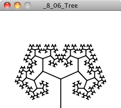
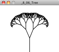
The recursive tree fractal is a nice example of a scenario in which adding a little bit of randomness can make the tree look more natural. Take a look outside and you’ll notice that branch lengths and angles vary from branch to branch, not to mention the fact that branches don’t all have exactly the same number of smaller branches. First, let’s see what happens when we simply vary the angle and length. This is a pretty easy one, given that we can just ask Processing for a random number each time we draw the tree.
void branch(float len) { float theta = random(0,PI/3);
line(0, 0, 0, -len);
translate(0, -len);
len *= 0.66;
if (len > 2) {
pushMatrix();
rotate(theta);
branch(len);
popMatrix();
pushMatrix();
rotate(-theta);
branch(len);
popMatrix();
}
}
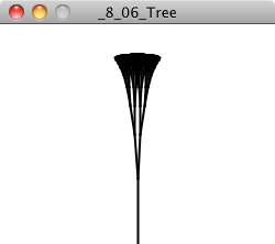
In the above function, we always call branch() twice. But why not pick a random number of branches and call branch() that number of times?
void branch(float len) {

  line(0, 0, 0, -len);
  translate(0, -len);

  if (len > 2) {
    int n = int(random(1,4));
    for (int i = 0; i < n; i++) {
      float theta = random(-PI/2, PI/2);
      pushMatrix();
      rotate(theta);
      branch(h);
      popMatrix();
    }
  }
Exercise 8.10
Set the angles of the branches of the tree according to Perlin noise values. Adjust the noise values over time to animate the tree. See if you can get it to appear as if it is blowing in the wind.
Exercise 8.11
Use toxiclibs to simulate tree physics. Each branch of the tree should be two particles connected with a spring. How can you get the tree to stand up and not fall down?
8.6 L-systems
In 1968, Hungarian botanist Aristid Lindenmayer developed a grammar-based system to model the growth patterns of plants. L-systems (short for Lindenmayer systems) can be used to generate all of the recursive fractal patterns we’ve seen so far in this chapter. We don’t need L-systems to do the kind of work we’re doing here; however, they are incredibly useful because they provide a mechanism for keeping track of fractal structures that require complex and multi-faceted production rules.
In order to create an example that implements L-systems in Processing, we are going to have to be comfortable with working with (a) recursion, (b) transformation matrices, and (c) strings. So far we’ve worked with recursion and transformations, but strings are new here. We will assume the basics, but if that is not comfortable for you, I would suggest taking a look at the Processing tutorial Strings and Drawing Text.
An L-system involves three main components:
Alphabet. An L-system’s alphabet is comprised of the valid characters that can be included. For example, we could say the alphabet is “ABC,” meaning that any valid “sentence” (a string of characters) in an L-system can only include these three characters.
Axiom. The axiom is a sentence (made up with characters from the alphabet) that describes the initial state of the system. For example, with the alphabet “ABC,” some example axioms are “AAA” or “B” or “ACBAB.”
Rules. The rules of an L-system are applied to the axiom and then applied recursively, generating new sentences over and over again. An L-system rule includes two sentences, a “predecessor” and a “successor.” For example, with the Rule “A —> AB”, whenever an “A” is found in a string, it is replaced with “AB.”
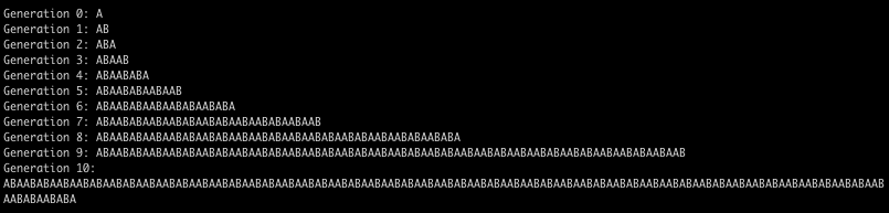
Let’s begin with a very simple L-system. (This is, in fact, Lindenmayer’s original L-system for modeling the growth of algae.)
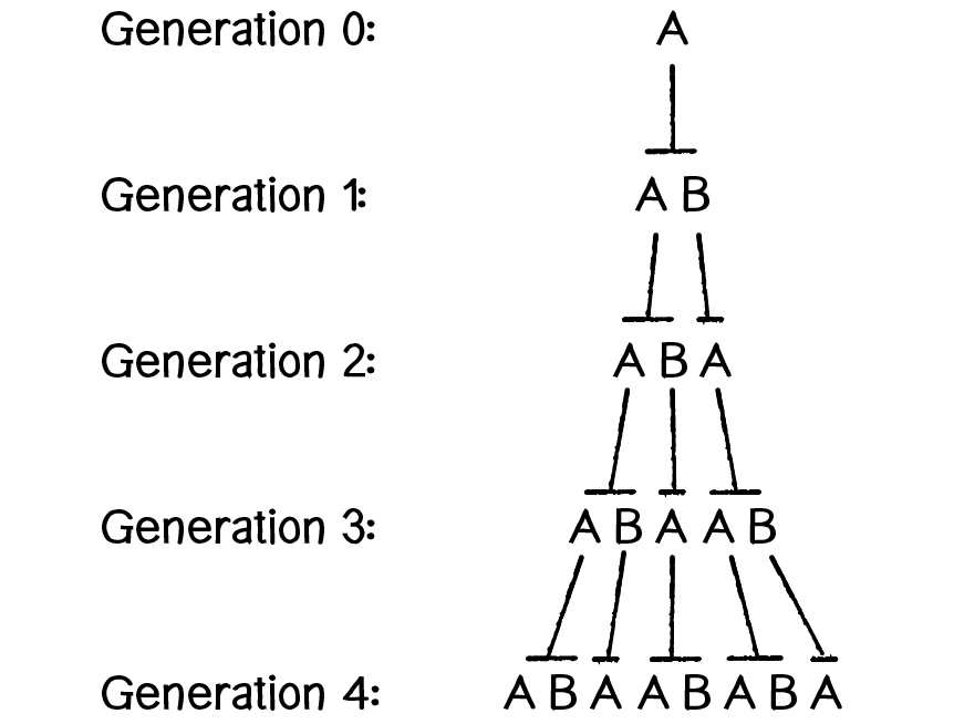
Figure 8.24: And so on and so forth...
Alphabet: A B
Axiom: A
Rules: (A → AB) (B → A)
As with our recursive fractal shapes, we can consider each successive application of the L-system rules to be a generation. Generation 0 is, by definition, the axiom.
Let’s look at how we might create these generations with code. We’ll start by using a String object to store the axiom.
String current = "A";And once again, just as we did with the Game of Life and the Koch curve ArrayList examples, we will need an entirely separate string to keep track of the “next” generation.
String next = "";Now it’s time to apply the rules to the current generation and place the results in the next.
for (int i = 0; i < current.length(); i++) {
  char c = current.charAt(i);
  if (c == 'A') {
    next += "AB";
  } else if (c == 'B') {
    next += "A";
  }
}
And when we’re done, current can become next.
current = next;To be sure this is working, let’s package it into a function and and call it every time the mouse is pressed.
Example 8.9: Simple L-system sentence generation
String current = "A";int count = 0;
void setup() {
println("Generation " + count + ": " + current);
}
void draw() {
}
void mousePressed() {
String next = "";
  for (int i = 0; i < current.length(); i++) {
    char c = current.charAt(i);
    if (c == 'A') {
      next += "AB";
    }  else if (c == 'B') {
      next += "A";
    }
  }
  current = next;
  count++;
  println("Generation " + count + ": " + current);
}
Since the rules are applied recursively to each generation, the length of the string grows exponentially. By generation #11, the sentence is 233 characters long; by generation #22, it is over 46,000 characters long. The Java String class, while convenient to use, is a grossly inefficient data structure for concatenating large strings. A String object is “immutable,” which means once the object is created it can never be changed. Whenever you add on to the end of a String object, Java has to make a brand new String object (even if you are using the same variable name).
String s = "blah";
s += "add some more stuff";
In most cases, this is fine, but why duplicate a 46,000-character string if you don’t have to? For better efficiency in our L-system examples, we’ll use the StringBuffer class, which is optimized for this type of task and can easily be converted into a string after concatenation is complete.
  StringBuffer next = new StringBuffer();
  for (int i = 0; i < current.length(); i++) {
    char c = current.charAt(i);
    if (c == 'A') {
      next.append("AB");
    } else if (c == 'B') {
      next.append("A");
    }
  }
current = next.toString();You may find yourself wondering right about now: what exactly is the point of all this? After all, isn’t this a chapter about drawing fractal patterns? Yes, the recursive nature of the L-system sentence structure seems relevant to the discussion, but how exactly does this model plant growth in a visual way?
What we’ve left unsaid until now is that embedded into these L-system sentences are instructions for drawing. Let’s see how this works with another example.
Alphabet: A B
Axiom: A
Rules: (A → ABA) (B → BBB)
To read a sentence, we’ll translate it in the following way:
A: Draw a line forward.
B: Move forward without drawing.
Let’s look at the sentence of each generation and its visual output.
Generation 0: A
Generation 1: ABA
Generation 2: ABABBBABA
Generation 3: ABABBBABABBBBBBBBBABABBBABA
Look familiar? This is the Cantor set generated with an L-system.

Figure 8.25
The following alphabet is often used with L-systems: “FG+-[]”, meaning:
F: Draw a line and move forward
G: Move forward (without drawing a line)
+: Turn right
-: Turn left
[: Save current location
]: Restore previous location
This type of drawing framework is often referred to as “Turtle graphics” (from the old days of LOGO programming). Imagine a turtle sitting on your computer screen to which you could issue a small set of commands: turn left, turn right, draw a line, etc. Processing isn’t set up to operate this way by default, but by using translate(), rotate(), and line(), we can emulate a Turtle graphics engine fairly easily.
Here’s how we would translate the above L-system alphabet into Processing code.
F: line(0,0,0,len); translate(0,len);
G: translate(0,len);
+: rotate(angle);
-: rotate(-angle);
[: pushMatrix();
]: popMatrix();
Assuming we have a sentence generated from the L-system, we can walk through the sentence character by character and call the appropriate function as outlined above.
for (int i = 0; i < sentence.length(); i++) {
char c = sentence.charAt(i);
  if (c == 'F') {
    line(0,0,len,0);
    translate(len,0);
  } else if (c == 'F') {
   translate(len,0);
  } else if (c == '+') {
    rotate(theta);
  } else if (c == '-') {
    rotate(-theta);
  } else if (c == '[') {
    pushMatrix();
  } else if (c == ']') {
    popMatrix();
  }
}The next example will draw a more elaborate structure with the following L-system.
Alphabet: FG+-[]
Axiom: F
Rules: F -→ FF+[+F-F-F]-[-F+F+F]
The example available for download on the book’s website takes all of the L-system code provided in this section and organizes it into three classes:
Rule: A class that stores the predecessor and successor strings for an L-system rule.
LSystem: A class to iterate a new L-system generation (as demonstrated with the StringBuffer technique).
Turtle: A class to manage reading the L-system sentence and following its instructions to draw on the screen.
We won’t write out these classes here since they simply duplicate the code we’ve already worked out in this chapter. However, let’s see how they are put together in the main tab.

LSystem lsys;
Turtle turtle;

void setup() {
  size(600,600);
  Rule[] ruleset = new Rule[1];
  ruleset[0] = new Rule('F',"FF+[+F-F-F]-[-F+F+F]");
lsys = new LSystem("F",ruleset);
  turtle = new Turtle(lsys.getSentence(),width/4,radians(25));
}

void draw() {
  background(255);
  translate(width/2,height);
  turtle.render();
}

void mousePressed() {
  lsys.generate();
  turtle.setToDo(lsys.getSentence());
  turtle.changeLen(0.5);
}
Exercise 8.12
Use an L-system as a set of instructions for creating objects stored in an ArrayList. Use trigonometry and vector math to perform the rotations instead of matrix transformations (much like we did in the Koch curve example).
Exercise 8.13
The seminal work in L-systems and plant structures, The Algorithmic Beauty of Plants by Przemysław Prusinkiewicz and Aristid Lindenmayer, was published in 1990. It is available for free in its entirety online. Chapter 1 describes many sophisticated L-systems with additional drawing rules and available alphabet characters. In addition, it describes several methods for generating stochastic L-systems. Expand the L-system example to include one or more additional features described by Prusinkiewicz and Lindenmayer.
Exercise 8.14
In this chapter, we emphasized using fractal algorithms for generating visual patterns. However, fractals can be found in other creative mediums. For example, fractal patterns are evident in Johann Sebastian Bach’s Cello Suite no. 3. The structure of David Foster Wallace’s novel Infinite Jest was inspired by fractals. Consider using the examples in this chapter to generate audio or text.
The Ecosystem Project
Step 8 Exercise:
Incorporate fractals into your ecosystem. Some possibilities:
Add plant-like creatures to the ecosystem environment.
Let’s say one of your plants is similar to a tree. Can you add leaves or flowers to the end of the branches? What if the leaves can fall off the tree (depending on a wind force)? What if you add fruit that can be picked and eaten by the creatures?
Design a creature with a fractal pattern.
Use an L-system to generate instructions for how a creature should move or behave.


void someFunction() {