Chapter 9. The Evolution of Code
“The fact that life evolved out of nearly nothing, some 10 billion years after the universe evolved out of literally nothing, is a fact so staggering that I would be mad to attempt words to do it justice.” — Richard Dawkins
Let’s take a moment to think back to a simpler time, when you wrote your first Processing sketches and life was free and easy. What is one of programming’s fundamental concepts that you likely used in those first sketches and continue to use over and over again? Variables. Variables allow you to save data and reuse that data while a program runs. This, of course, is nothing new to us. In fact, we have moved far beyond a sketch with just one or two variables and on to more complex data structures—variables made from custom types (objects) that include both data and functionality. We’ve made our own little worlds of movers and particles and vehicles and cells and trees.
In each and every example in this book, the variables of these objects have to be initialized. Perhaps you made a whole bunch of particles with random colors and sizes or a list of vehicles all starting at the same x,y location on screen. But instead of acting as “intelligent designers” and assigning the properties of our objects through randomness or thoughtful consideration, we can let a process found in nature—evolution—decide for us.
Can we think of the variables of an object as its DNA? Can objects make other objects and pass down their DNA to a new generation? Can our simulation evolve?
The answer to all these questions is yes. After all, we wouldn’t be able to face ourselves in the mirror as nature-of-coders without tackling a simulation of one of the most powerful algorithmic processes found in nature itself. This chapter is dedicated to examining the principles behind biological evolution and finding ways to apply those principles in code.
9.1 Genetic Algorithms: Inspired by Actual Events
It’s important for us to clarify the goals of this chapter. We will not go into depth about the science of genetics and evolution as it happens in the real world. We won’t be making Punnett squares (sorry to disappoint) and there will be no discussion of nucleotides, protein synthesis, RNA, and other topics related to the actual biological processes of evolution. Instead, we are going to look at the core principles behind Darwinian evolutionary theory and develop a set of algorithms inspired by these principles. We don’t care so much about an accurate simulation of evolution; rather, we care about methods for applying evolutionary strategies in software.
This is not to say that a project with more scientific depth wouldn’t have value, and I encourage readers with a particular interest in this topic to explore possibilities for expanding the examples provided with additional evolutionary features. Nevertheless, for the sake of keeping things manageable, we’re going to stick to the basics, which will be plenty complex and exciting.
The term “genetic algorithm” refers to a specific algorithm implemented in a specific way to solve specific sorts of problems. While the formal genetic algorithm itself will serve as the foundation for the examples we create in this chapter, we needn’t worry about implementing the algorithm with perfect accuracy, given that we are looking for creative uses of evolutionary theories in our code. This chapter will be broken down into the following three parts (with the majority of the time spent on the first).
Traditional Genetic Algorithm. We’ll begin with the traditional computer science genetic algorithm. This algorithm was developed to solve problems in which the solution space is so vast that a “brute force” algorithm would simply take too long. Here’s an example: I’m thinking of a number. A number between one and one billion. How long will it take for you to guess it? Solving a problem with “brute force” refers to the process of checking every possible solution. Is it one? Is it two? Is it three? Is it four? And so and and so forth. Though luck does play a factor here, with brute force we would often find ourselves patiently waiting for years while you count to one billion. However, what if I could tell you if an answer you gave was good or bad? Warm or cold? Very warm? Hot? Super, super cold? If you could evaluate how “fit” a guess is, you could pick other numbers closer to that guess and arrive at the answer more quickly. Your answer could evolve.
Interactive Selection. Once we establish the traditional computer science algorithm, we’ll look at other applications of genetic algorithms in the visual arts. Interactive selection refers to the process of evolving something (often an computer-generated image) through user interaction. Let’s say you walk into a museum gallery and see ten paintings. With interactive selection, you would pick your favorites and allow an algorithmic process to generate (or “evolve”) new paintings based on your preferences.
Ecosystem Simulation. The traditional computer science genetic algorithm and interactive selection technique are what you will likely find if you search online or read a textbook about artificial intelligence. But as we’ll soon see, they don’t really simulate the process of evolution as it happens in the real world. In this chapter, I want to also explore techniques for simulating the process of evolution in an ecosystem of pseudo-living beings. How can our objects that move about the screen meet each other, mate, and pass their genes on to a new generation? This would apply directly to the Ecosystem Project outlined at the end of each chapter.
9.2 Why Use Genetic Algorithms?
While computer simulations of evolutionary processes date back to the 1950s, much of what we think of as genetic algorithms (also known as “GAs”) today was developed by John Holland, a professor at the University of Michigan, whose book Adaptation in Natural and Artificial Systems pioneered GA research. Today, more genetic algorithms are part of a wider field of research, often referred to as "Evolutionary Computing."
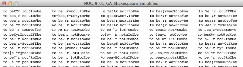
To help illustrate the traditional genetic algorithm, we are going to start with monkeys. No, not our evolutionary ancestors. We’re going to start with some fictional monkeys that bang away on keyboards with the goal of typing out the complete works of Shakespeare.
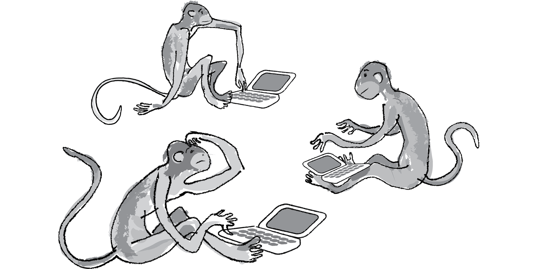
Figure 9.1
The “infinite monkey theorem” is stated as follows: A monkey hitting keys randomly on a typewriter will eventually type the complete works of Shakespeare (given an infinite amount of time). The problem with this theory is that the probability of said monkey actually typing Shakespeare is so low that even if that monkey started at the Big Bang, it’s unbelievably unlikely we’d even have Hamlet at this point.
Let’s consider a monkey named George. George types on a reduced typewriter containing only twenty-seven characters: twenty-six letters and one space bar. So the probability of George hitting any given key is one in twenty-seven.
Let’s consider the phrase “to be or not to be that is the question” (we’re simplifying it from the original “To be, or not to be: that is the question”). The phrase is 39 characters long. If George starts typing, the chance he’ll get the first character right is 1 in 27. Since the probability he’ll get the second character right is also 1 in 27, he has a 1 in 27*27 chance of landing the first two characters in correct order—which follows directly from our discussion of "event probability" in the Introduction. Therefore, the probability that George will type the full phrase is:
(1/27) multiplied by itself 39 times, i.e. (1/27)39
which equals a 1 in 66,555,937,033,867,822,607,895,549,241,096,482,953,017,615,834,735,226,163 chance of getting it right!
Needless to say, even hitting just this one phrase, not to mention an entire play, is highly unlikely. Even if George is a computer simulation and can type one million random phrases per second, for George to have a 99% probability of eventually getting it right, he would have to type for 9,719,096,182,010,563,073,125,591,133,903,305,625,605,017 years. (Note that the age of the universe is estimated to be a mere 13,750,000,000 years.)
The point of all these unfathomably large numbers is not to give you a headache, but to demonstrate that a brute force algorithm (typing every possible random phrase) is not a reasonable strategy for arriving randomly at “to be or not to be that is the question”. Enter genetic algorithms, which will show that we can still start with random phrases and find the solution through simulated evolution.
Now, it’s worth noting that this problem (arrive at the phrase “to be or not to be that is the question”) is a ridiculous one. Since we know the answer, all we need to do is type it. Here’s a Processing sketch that solves the problem.
Nevertheless, the point here is that solving a problem with a known answer allows us to easily test our code. Once we’ve successfully solved the problem, we can feel more confident in using genetic algorithms to do some actual useful work: solving problems with unknown answers. So this first example serves no real purpose other than to demonstrate how genetic algorithms work. If we test the GA results against the known answer and get “to be or not to be”, then we’ve succeeded in writing our genetic algorithm.
Exercise 9.1
Create a sketch that generates random strings. We’ll need to know how to do this in order to implement the genetic algorithm example that will shortly follow. How long does it take for Processing to randomly generate the string “cat”? How could you adapt this to generate a random design using Processing’s shape-drawing functions?
9.3 Darwinian Natural Selection
Before we begin walking through the genetic algorithm, let’s take a moment to describe three core principles of Darwinian evolution that will be required as we implement our simulation. In order for natural selection to occur as it does in nature, all three of these elements must be present.
Heredity. There must be a process in place by which children receive the properties of their parents. If creatures live long enough to reproduce, then their traits are passed down to their children in the next generation of creatures.
Variation. There must be a variety of traits present in the population or a means with which to introduce variation. For example, let’s say there is a population of beetles in which all the beetles are exactly the same: same color, same size, same wingspan, same everything. Without any variety in the population, the children will always be identical to the parents and to each other. New combinations of traits can never occur and nothing can evolve.
Selection. There must be a mechanism by which some members of a population have the opportunity to be parents and pass down their genetic information and some do not. This is typically referred to as “survival of the fittest.” For example, let’s say a population of gazelles is chased by lions every day. The faster gazelles are more likely to escape the lions and are therefore more likely to live longer and have a chance to reproduce and pass their genes down to their children. The term fittest, however, can be a bit misleading. Generally, we think of it as meaning bigger, faster, or stronger. While this may be the case in some instances, natural selection operates on the principle that some traits are better adapted for the creature’s environment and therefore produce a greater likelihood of surviving and reproducing. It has nothing to do with a given creature being “better” (after all, this is a subjective term) or more “physically fit.” In the case of our typing monkeys, for example, a more “fit” monkey is one that has typed a phrase closer to “to be or not to be”.
Next I’d like to walk through the narrative of the genetic algorithm. We’ll do this in the context of the typing monkey. The algorithm itself will be divided into two parts: a set of conditions for initialization (i.e. Processing’s setup()) and the steps that are repeated over and over again (i.e. Processing’s draw()) until we arrive at the correct answer.
9.4 The Genetic Algorithm, Part I: Creating a Population
In the context of the typing monkey example, we will create a population of phrases. (Note that we are using the term “phrase” rather loosely, meaning a string of characters.) This begs the question: How do we create this population? Here is where the Darwinian principle of variation applies. Let’s say, for simplicity, that we are trying to evolve the phrase “cat” and that we have a population of three phrases.
hug
rid
won
Sure, there is variety in the three phrases above, but try to mix and match the characters every which way and you will never get cat. There is not enough variety here to evolve the optimal solution. However, if we had a population of thousands of phrases, all generated randomly, chances are that at least one member of the population will have a c as the first character, one will have an a as the second, and one a t as the third. A large population will most likely give us enough variety to generate the desired phrase (and in Part 2 of the algorithm, we’ll have another opportunity to introduce even more variation in case there isn’t enough in the first place). So we can be more specific in describing Step 1 and say:
Create a population of randomly generated elements.
This brings up another important question. What is the element itself? As we move through the examples in this chapter, we’ll see several different scenarios; we might have a population of images or a population of vehicles à la Chapter 6. The key, and the part that is new for us in this chapter, is that each member of the population has a virtual “DNA,” a set of properties (we can call them “genes”) that describe how a given element looks or behaves. In the case of the typing monkey, for example, the DNA is simply a string of characters.
In the field of genetics, there is an important distinction between the concepts genotype and phenotype. The actual genetic code—in our case, the digital information itself—is an element’s genotype. This is what gets passed down from generation to generation. The phenotype, however, is the expression of that data. This distinction is key to how you will use genetic algorithms in your own work. What are the objects in your world? How will you design the genotype for your objects (the data structure to store each object’s properties) as well as the phenotype (what are you using these variables to express?) We do this all the time in graphics programming. The simplest example is probably color.
| Genotype | Phenotype |
|---|---|
| int c = 255; | |
| int c = 127; | |
| int c = 0; |
As we can see, the genotype is the digital information. Each color is a variable that stores an integer and we choose to express that integer as a color. But how we choose to express the data is arbitrary. In a different approach, we could have used the integer to describe the length of a line, the weight of a force, etc.
| Same Genotype | Different Phenotype (line length) |
|---|---|
| int c = 255; | |
| int c = 127; | |
| int c = 0; |
The nice thing about our monkey-typing example is that there is no difference between genotype and phenotype. The DNA data itself is a string of characters and the expression of that data is that very string.
So, we can finally end the discussion of this first step and be more specific with its description, saying:
Create a population of N elements, each with randomly generated DNA.
9.5 The Genetic Algorithm, Part II: Selection
Here is where we apply the Darwinian principle of selection. We need to evaluate the population and determine which members are fit to be selected as parents for the next generation. The process of selection can be divided into two steps.
1) Evaluate fitness.
For our genetic algorithm to function properly, we will need to design what is referred to as a fitness function. The function will produce a numeric score to describe the fitness of a given member of the population. This, of course, is not how the real world works at all. Creatures are not given a score; they simply survive or not. But in the case of the traditional genetic algorithm, where we are trying to evolve an optimal solution to a problem, we need to be able to numerically evaluate any given possible solution.
Let’s examine our current example, the typing monkey. Again, let’s simplify the scenario and say we are attempting to evolve the word “cat”. We have three members of the population: hut, car, and box. Car is obviously the most fit, given that it has two correct characters, hut has only one, and box has zero. And there it is, our fitness function:
fitness = the number of correct characters
| DNA | Fitness |
|---|---|
hut |
1 |
car |
2 |
box |
0 |
We will eventually want to look at examples with more sophisticated fitness functions, but this is a good place to start.
2) Create a mating pool.
Once the fitness has been calculated for all members of the population, we can then select which members are fit to become parents and place them in a mating pool. There are several different approaches we could take here. For example, we could employ what is known as the elitist method and say, “Which two members of the population scored the highest? You two will make all the children for the next generation.” This is probably one of the easier methods to program; however, it flies in the face of the principle of variation. If two members of the population (out of perhaps thousands) are the only ones available to reproduce, the next generation will have little variety and this may stunt the evolutionary process. We could instead make a mating pool out of a larger number—for example, the top 50% of the population, 500 out of 1,000. This is also just as easy to program, but it will not produce optimal results. In this case, the high-scoring top elements would have the same chance of being selected as a parent as the ones toward the middle. And why should element number 500 have a solid shot of reproducing, while element number 501 has no shot?
A better solution for the mating pool is to use a probabilistic method, which we’ll call the “wheel of fortune” (also known as the “roulette wheel”). To illustrate this method, let’s consider a simple example where we have a population of five elements, each with a fitness score.
| Element | Fitness |
|---|---|
A |
3 |
B |
4 |
C |
0.5 |
D |
1.5 |
E |
1 |
The first thing we’ll want to do is normalize all the scores. Remember normalizing a vector? That involved taking an vector and standardizing its length, setting it to 1. When we normalize a set of fitness scores, we are standardizing their range to between 0 and 1, as a percentage of total fitness. Let’s add up all the fitness scores.
total fitness = 3 + 4 + 0.5 + 1.5 + 1 = 10
Then let’s divide each score by the total fitness, giving us the normalized fitness.
| Element | Fitness | Normalized Fitness | Expressed as a Percentage |
|---|---|---|---|
A |
3 |
0.3 |
30% |
B |
4 |
0.4 |
40% |
C |
0.5 |
0.05 |
5% |
D |
1.5 |
0.15 |
15% |
E |
1 |
0.1 |
10% |
Now it’s time for the wheel of fortune.
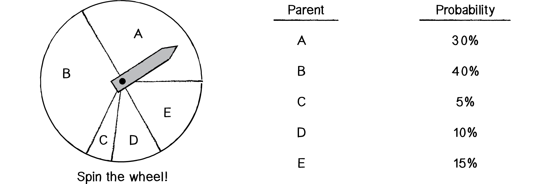
Figure 9.2
Spin the wheel and you’ll notice that Element B has the highest chance of being selected, followed by A, then D, then E, and finally C. This probability-based selection according to fitness is an excellent approach. One, it guarantees that the highest-scoring elements will be most likely to reproduce. Two, it does not entirely eliminate any variation from the population. Unlike with the elitist method, even the lowest-scoring element (in this case C) has a chance to pass its information down to the next generation. It’s quite possible (and often the case) that even low-scoring elements have a tiny nugget of genetic code that is truly useful and should not entirely be eliminated from the population. For example, in the case of evolving “to be or not to be”, we might have the following elements.
A: to be or not to go
B: to be or not to pi
C: xxxxxxxxxxxxxxxxbe
As you can see, elements A and B are clearly the most fit and would have the highest score. But neither contains the correct characters for the end of the phrase. Element C, even though it would receive a very low score, happens to have the genetic data for the end of the phrase. And so while we would want A and B to be picked to generate the majority of the next generation, we would still want C to have a small chance to participate in the reproductive process.
9.6 The Genetic Algorithm, Part III: Reproduction
Now that we have a strategy for picking parents, we need to figure out how to use reproduction to make the population’s next generation, keeping in mind the Darwinian principle of heredity—that children inherit properties from their parents. Again, there are a number of different techniques we could employ here. For example, one reasonable (and easy to program) strategy is asexual reproduction, meaning we pick just one parent and create a child that is an exact copy of that parent. The standard approach with genetic algorithms, however, is to pick two parents and create a child according to the following steps.
1) Crossover.
Crossover involves creating a child out of the genetic code of two parents. In the case of the monkey-typing example, let’s assume we’ve picked two phrases from the mating pool (as outlined in our selection step).
Parent A: FORK
Parent B: PLAY
It’s now up to us to make a child phrase from these two. Perhaps the most obvious way (let’s call this the 50/50 method) would be to take the first two characters from A and the second two from B, leaving us with:
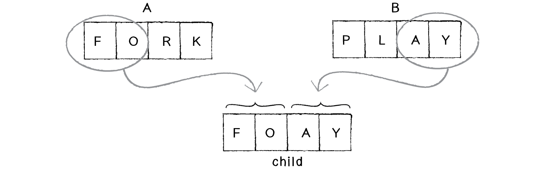
Figure 9.3
A variation of this technique is to pick a random midpoint. In other words, we don’t have to pick exactly half of the code from each parent. We could sometimes end up with FLAY, and sometimes with FORY. This is preferable to the 50/50 approach, since we increase the variety of possibilities for the next generation.
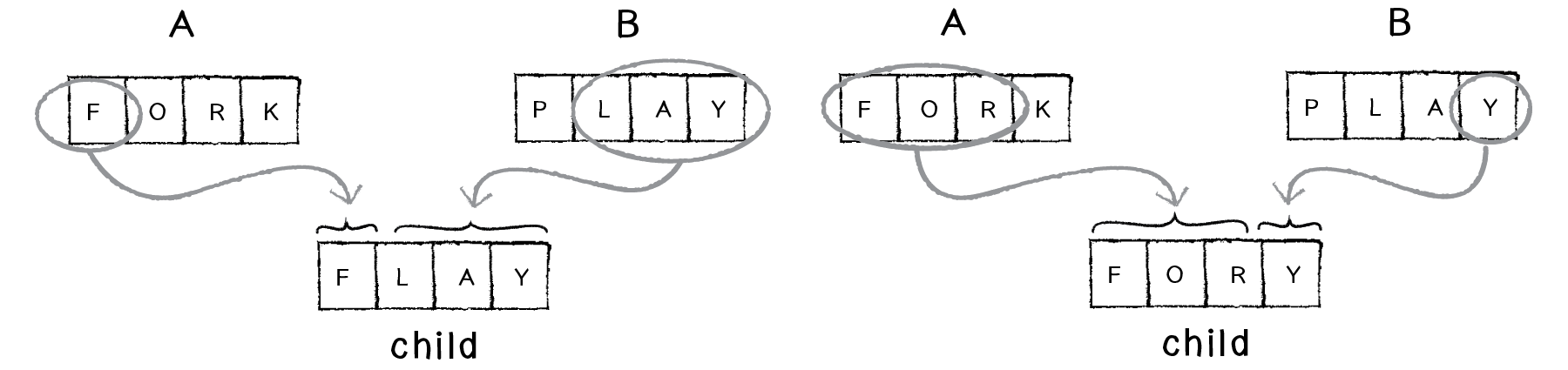
Figure 9.4: Picking a random midpoint
Another possibility is to randomly select a parent for each character in the child string. You can think of this as flipping a coin four times: heads take from parent A, tails from parent B. Here we could end up with many different results such as: PLRY, FLRK, FLRY, FORY, etc.
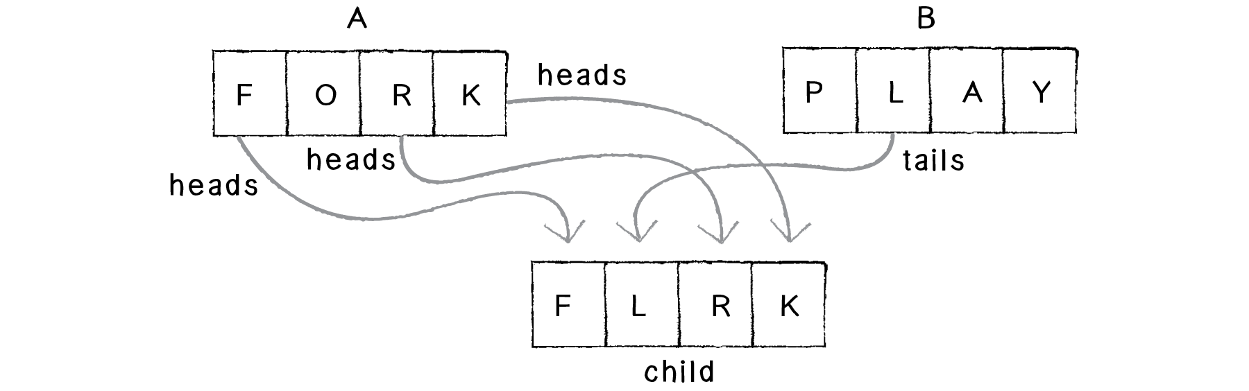
Figure 9.5: Coin-flipping approach
This strategy will produce essentially the same results as the random midpoint method; however, if the order of the genetic information plays some role in expressing the phenotype, you may prefer one solution over the other.
2) Mutation.
Once the child DNA has been created via crossover, we apply one final process before adding the child to the next generation—mutation. Mutation is an optional step, as there are some cases in which it is unnecessary. However, it exists because of the Darwinian principle of variation. We created an initial population randomly, making sure that we start with a variety of elements. However, there can only be so much variety when seeding the first generation, and mutation allows us to introduce additional variety throughout the evolutionary process itself.
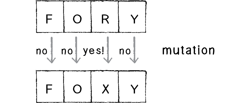
Figure 9.6
Mutation is described in terms of a rate. A given genetic algorithm might have a mutation rate of 5% or 1% or 0.1%, etc. Let’s assume we just finished with crossover and ended up with the child FORY. If we have a mutation rate of 1%, this means that for each character in the phrase generated from crossover, there is a 1% chance that it will mutate. What does it mean for a character to mutate? In this case, we define mutation as picking a new random character. A 1% probability is fairly low, and most of the time mutation will not occur at all in a four-character string (96% of the time to be more precise). However, when it does, the mutated character is replaced with a randomly generated one (see Figure 9.6).
As we’ll see in some of the examples, the mutation rate can greatly affect the behavior of the system. Certainly, a very high mutation rate (such as, say, 80%) would negate the evolutionary process itself. If the majority of a child’s genes are generated randomly, then we cannot guarantee that the more “fit” genes occur with greater frequency with each successive generation.
The process of selection (picking two parents) and reproduction (crossover and mutation) is applied over and over again N times until we have a new population of N elements. At this point, the new population of children becomes the current population and we loop back to evaluate fitness and perform selection and reproduction again.
Now that we have described all the steps of the genetic algorithm in detail, it’s time to translate these steps into Processing code. Because the previous description was a bit longwinded, let’s look at an overview of the algorithm first. We’ll then cover each of the three steps in its own section, working out the code.
SETUP:
Step 1: Initialize. Create a population of N elements, each with randomly generated DNA.
LOOP:
Step 2: Selection. Evaluate the fitness of each element of the population and build a mating pool.
Step 3: Reproduction. Repeat N times:
a) Pick two parents with probability according to relative fitness.
b) Crossover—create a “child” by combining the DNA of these two parents.
c) Mutation—mutate the child’s DNA based on a given probability.
d) Add the new child to a new population.
Step 4. Replace the old population with the new population and return to Step 2.
9.7 Code for Creating the Population
Step 1: Initialize Population
If we’re going to create a population, we need a data structure to store a list of members of the population. In most cases (such as our typing-monkey example), the number of elements in the population can be fixed, and so we use an array. (Later we’ll see examples that involve a growing/shrinking population and we’ll use an ArrayList.) But an array of what? We need an object that stores the genetic information for a member of the population. Let’s call it DNA.
class DNA {

}
The population will then be an array of DNA objects.
DNA[] population = new DNA[100];But what stuff goes in the DNA class? For a typing monkey, its DNA is the random phrase it types, a string of characters.
class DNA {
  String phrase;
}
While this is perfectly reasonable for this particular example, we’re not going to use an actual String object as the genetic code. Instead, we’ll use an array of characters.
class DNA { char[] genes = new char[18];
}
By using an array, we’ll be able to extend all the code we write into other examples. For example, the DNA of a creature in a physics system might be an array of PVectors—or for an image, an array of integers (RGB colors). We can describe any set of properties in an array, and even though a string is convenient for this particular sketch, an array will serve as a better foundation for future evolutionary examples.
Our genetic algorithm dictates that we create a population of N elements, each with randomly generated DNA. Therefore, in the object’s constructor, we randomly create each character of the array.
class DNA {
  char[] genes = new char[18];

  DNA() {
    for (int i = 0; i < genes.length; i++) {
      genes[i] = (char) random(32,128);
    }
  }
}
Now that we have the constructor, we can return to setup() and initialize each DNA object in the population array.
DNA[] population = new DNA[100];

void setup() {
  for (int i = 0; i < population.length; i++) {
    population[i] = new DNA();
  }
}
Our DNA class is not at all complete. We’ll need to add functions to it to perform all the other tasks in our genetic algorithm, which we’ll do as we walk through steps 2 and 3.
Step 2: Selection
Step 2 reads, “Evaluate the fitness of each element of the population and build a mating pool.” Let’s first evaluate each object’s fitness. Earlier we stated that one possible fitness function for our typed phrases is the total number of correct characters. Let’s revise this fitness function a little bit and state it as the percentage of correct characters—i.e., the total number of correct characters divided by the total characters.
Fitness = Total # Characters Correct/Total # Characters
Where should we calculate the fitness? Since the DNA class contains the genetic information (the phrase we will test against the target phrase), we can write a function inside the DNA class itself to score its own fitness. Let’s assume we have a target phrase:
String target = "to be or not to be";We can now compare each “gene” against the corresponding character in the target phrase, incrementing a counter each time we get a correct character.
class DNA { float fitness;
  void fitness () {
    int score = 0;
    for (int i = 0; i < genes.length; i++) {
if (genes[i] == target.charAt(i)) { score++;
}
}
fitness = float(score)/target.length();
}
In the main tab’s draw(), the very first step we’ll take is to call the fitness function for each member of the population.
void draw() {
for (int i = 0; i < population.length; i++) {
population[i].fitness();
}
After we have all the fitness scores, we can build the “mating pool” that we’ll need for the reproduction step. The mating pool is a data structure from which we’ll continuously pick two parents. Recalling our description of the selection process, we want to pick parents with probabilities calculated according to fitness. In other words, the members of the population that have the highest fitness scores should be most likely to be picked; those with the lowest scores, the least likely.
In the Introduction, we covered the basics of probability and generating a custom distribution of random numbers. We’re going to use those techniques to assign a probability to each member of the population, picking parents by spinning the “wheel of fortune.” Let’s look at Figure 9.2 again.
Figure 9.2 (again)
It might be fun to do something ridiculous and actually program a simulation of a spinning wheel as depicted above. But this is quite unnecessary.
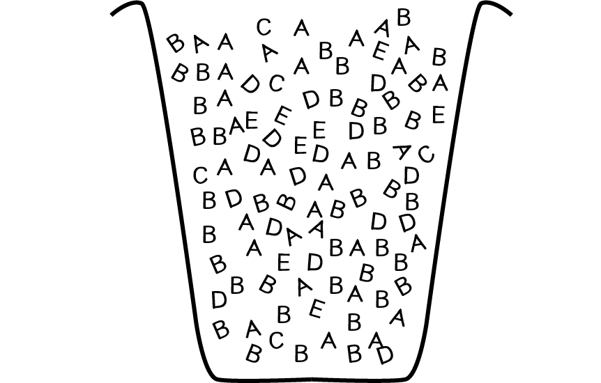
Figure 9.7
Instead we can pick from the five options (ABCDE) according to their probabilities by filling an ArrayList with multiple instances of each parent. In other words, let’s say you had a bucket of wooden letters—30 As, 40 Bs, 5 Cs, 15 Ds, and 10 Es.
If you pick a random letter out of that bucket, there’s a 30% chance you’ll get an A, a 5% chance you’ll get a C, and so on. For us, that bucket is an ArrayList, and each wooden letter is a potential parent. We add each parent to the ArrayList N number of times where N is equal to its percentage score.
ArrayList<DNA> matingPool = new ArrayList<DNA>();
for (int i = 0; i < population.length; i++) {
int n = int(population[i].fitness * 100);
for (int j = 0; j < n; j++) {
matingPool.add(population[i]);
}
}
Exercise 9.2
One of the other methods we used to generate a custom distribution of random numbers is called the Monte Carlo method. This technique involved picking two random numbers, with the second number acting as a qualifying number and determining if the first random number should be kept or thrown away. Rewrite the above mating pool algorithm to use the Monte Carlo method instead.
Exercise 9.3
In some cases, the wheel of fortune algorithm will have an extraordinarily high preference for some elements over others. Take the following probabilities:
A: 98%
B: 1%
C: 1%
This is sometimes undesirable given how it will decrease the amount of variety in this system. A solution to this problem is to replace the calculated fitness scores with the ordinals of scoring (meaning their rank).
A: 50% (3/6)
B: 33% (2/6)
C: 17% (1/6)
Rewrite the mating pool algorithm to use this method instead.
Step 3: Reproduction
With the mating pool ready to go, it’s time to make some babies. The first step is to pick two parents. Again, it’s somewhat of an arbitrary decision to pick two parents. It certainly mirrors human reproduction and is the standard means in the traditional GA, but in terms of your work, there really aren’t any restrictions here. You could choose to perform “asexual” reproduction with one parent, or come up with a scheme for picking three or four parents from which to generate child DNA. For this code demonstration, we’ll stick to two parents and call them parentA and parentB.
First thing we need are two random indices into the mating pool—random numbers between 0 and the size of the ArrayList.
int a = int(random(matingPool.size()));
int b = int(random(matingPool.size()));
We can use these indices to retrieve an actual DNA instance from the mating pool.
DNA parentA = matingPool.get(a);
DNA parentB = matingPool.get(b);
Because we have multiple instances of the same DNA objects in the mating pool (not to mention that we could pick the same random number twice), it’s possible that parentA and parentB could be the same DNA object. If we wanted to be strict, we could write some code to ensure that we haven’t picked the same parent twice, but we would gain very little efficiency for all that extra code. Still, it‘s worth trying this as an exercise.
Once we have the two parents, we can perform crossover to generate the child DNA, followed by mutation.
DNA child = parentA.crossover(parentB); child.mutate();Of course, the functions crossover() and mutate() don’t magically exist in our DNA class; we have to write them. The way we called crossover() above indicates that the function receives an instance of DNA as an argument and returns a new instance of DNA, the child.
DNA crossover(DNA partner) {
DNA child = new DNA();
int midpoint = int(random(genes.length));
for (int i = 0; i < genes.length; i++) {
if (i > midpoint) child.genes[i] = genes[i];
else child.genes[i] = partner.genes[i];
}
return child;
}
The above crossover function uses the “random midpoint” method of crossover, in which the first section of genes is taken from parent A and the second section from parent B.
Exercise 9.5
Rewrite the crossover function to use the “coin flipping” method instead, in which each gene has a 50% chance of coming from parent A and a 50% chance of coming from parent B.
The mutate() function is even simpler to write than crossover(). All we need to do is loop through the array of genes and for each randomly pick a new character according to the mutation rate. With a mutation rate of 1%, for example, we would pick a new character one time out of a hundred.
float mutationRate = 0.01;
if (random(1) < mutationRate) {
}
The entire function therefore reads:
void mutate() { for (int i = 0; i < genes.length; i++) {
if (random(1) < mutationRate) {
genes[i] = (char) random(32,128);
}
}
}
9.8 Genetic Algorithms: Putting It All Together
You may have noticed that we’ve essentially walked through the steps of the genetic algorithm twice, once describing it in narrative form and another time with code snippets implementing each of the steps. What I’d like to do in this section is condense the previous two sections into one page, with the algorithm described in just three steps and the corresponding code alongside.
Example 9.1: Genetic algorithm: Evolving Shakespeare
float mutationRate;int totalPopulation = 150;
DNA[] population;ArrayList<DNA> matingPool;String target;
void setup() {
size(640, 360);
target = "to be or not to be";
mutationRate = 0.01;
population = new DNA[totalPopulation];
for (int i = 0; i < population.length; i++) {
population[i] = new DNA();
}
}
void draw() {
for (int i = 0; i < population.length; i++) {
population[i].fitness();
}
ArrayList<DNA> matingPool = new ArrayList<DNA>();
for (int i = 0; i < population.length; i++) {
int n = int(population[i].fitness * 100);
for (int j = 0; j < n; j++) {
matingPool.add(population[i]);
}
}
for (int i = 0; i < population.length; i++) {
int a = int(random(matingPool.size()));
int b = int(random(matingPool.size()));
DNA partnerA = matingPool.get(a);
DNA partnerB = matingPool.get(b);
DNA child = partnerA.crossover(partnerB); child.mutate(mutationRate);
population[i] = child;
}
}
The main tab precisely mirrors the steps of the genetic algorithm. However, most of the functionality called upon is actually present in the DNA class itself.
class DNA {
char[] genes;
float fitness;
DNA() {
genes = new char[target.length()];
for (int i = 0; i < genes.length; i++) {
genes[i] = (char) random(32,128);
}
}
void fitness() {
int score = 0;
for (int i = 0; i < genes.length; i++) {
if (genes[i] == target.charAt(i)) {
        score++;
      }
    }
    fitness = float(score)/target.length();
  }
DNA crossover(DNA partner) {
DNA child = new DNA(genes.length);
    int midpoint = int(random(genes.length));

    for (int i = 0; i < genes.length; i++) {
      if (i > midpoint) child.genes[i] = genes[i];
      else child.genes[i] = partner.genes[i];
}
    return child;
  }
void mutate(float mutationRate) {
    for (int i = 0; i < genes.length; i++) {
      if (random(1) < mutationRate) {
        genes[i] = (char) random(32,128);
      }
    }
  }
  String getPhrase() {
    return new String(genes);
  }
}
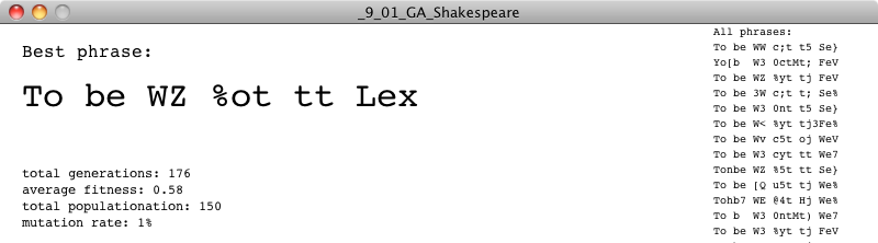
Exercise 9.6
Add features to the above example to report more information about the progress of the genetic algorithm itself. For example, show the phrase closest to the target each generation, as well as report on the number of generations, average fitness, etc. Stop the genetic algorithm once it has solved the phrase. Consider writing a Population class to manage the GA, instead of including all the code in draw().
9.9 Genetic Algorithms: Make Them Your Own
The nice thing about using genetic algorithms in a project is that example code can easily be ported from application to application. The core mechanics of selection and reproduction don’t need to change. There are, however, three key components to genetic algorithms that you, the developer, will have to customize for each use. This is crucial to moving beyond trivial demonstrations of evolutionary simulations (as in the Shakespeare example) to creative uses in projects that you make in Processing and other creative programming environments.
Key #1: Varying the variables
There aren’t a lot of variables to the genetic algorithm itself. In fact, if you look at the previous example’s code, you’ll see only two global variables (not including the arrays and ArrayLists to store the population and mating pool).
float mutationRate = 0.01;
int totalPopulation = 150;
These two variables can greatly affect the behavior of the system, and it’s not such a good idea to arbitrarily assign them values (though tweaking them through trial and error is a perfectly reasonable way to arrive at optimal values).
The values I chose for the Shakespeare demonstration were picked to virtually guarantee that the genetic algorithm would solve for the phrase, but not too quickly (approximately 1,000 generations on average) so as to demonstrate the process over a reasonable period of time. A much larger population, however, would yield faster results (if the goal were algorithmic efficiency rather than demonstration). Here is a table of some results.
| Total Population | Mutation Rate | Number of Generations until Phrase Solved | Total Time (in seconds) until Phrase Solved |
|---|---|---|---|
150 |
1% |
1089 |
18.8 |
300 |
1% |
448 |
8.2 |
1,000 |
1% |
71 |
1.8 |
50,000 |
1% |
27 |
4.3 |
Notice how increasing the population size drastically reduces the number of generations needed to solve for the phrase. However, it doesn’t necessarily reduce the amount of time. Once our population balloons to fifty thousand elements, the sketch runs slowly, given the amount of time required to process fitness and build a mating pool out of so many elements. (There are, of course, optimizations that could be made should you require such a large population.)
In addition to the population size, the mutation rate can greatly affect performance.
| Total Population | Mutation Rate | Number of Generations until Phrase Solved | Total Time (in seconds) until Phrase Solved |
|---|---|---|---|
1,000 |
0% |
37 or never? |
1.2 or never? |
1,000 |
1% |
71 |
1.8 |
1,000 |
2% |
60 |
1.6 |
1,000 |
10% |
never? |
never? |
Without any mutation at all (0%), you just have to get lucky. If all the correct characters are present somewhere in some member of the initial population, you’ll evolve the phrase very quickly. If not, there is no way for the sketch to ever reach the exact phrase. Run it a few times and you’ll see both instances. In addition, once the mutation rate gets high enough (10%, for example), there is so much randomness involved (1 out of every 10 letters is random in each new child) that the simulation is pretty much back to a random typing monkey. In theory, it will eventually solve the phrase, but you may be waiting much, much longer than is reasonable.
Key #2: The fitness function
Playing around with the mutation rate or population total is pretty easy and involves little more than typing numbers in your sketch. The real hard work of a developing a genetic algorithm is in writing a fitness function. If you cannot define your problem’s goals and evaluate numerically how well those goals have been achieved, then you will not have successful evolution in your simulation.
Before we think about other scenarios with other fitness functions, let’s look at flaws in our Shakespearean fitness function. Consider solving for a phrase that is not nineteen characters long, but one thousand. Now, let’s say there are two members of the population, one with 800 characters correct and one with 801. Here are their fitness scores:
Phrase A: |
800 characters correct |
fitness = 80% |
Phrase B: |
801 characters correct |
fitness = 80.1% |
There are a couple of problems here. First, we are adding elements to the mating pool N numbers of times, where N equals fitness multiplied by 100. Objects can only be added to an ArrayList a whole number of times, and so A and B will both be added 80 times, giving them an equal probability of being selected. Even with an improved solution that takes floating point probabilities into account, 80.1% is only a teeny tiny bit higher than 80%. But getting 801 characters right is a whole lot better than 800 in the evolutionary scenario. We really want to make that additional character count. We want the fitness score for 801 characters to be exponentially better than the score for 800.
To put it another way, let’s graph the fitness function.
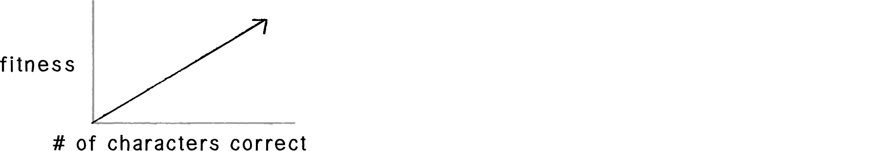
Figure 9.8
This is a linear graph; as the number of characters goes up, so does the fitness score. However, what if the fitness increased exponentially as the number of correct characters increased? Our graph could then look something like:
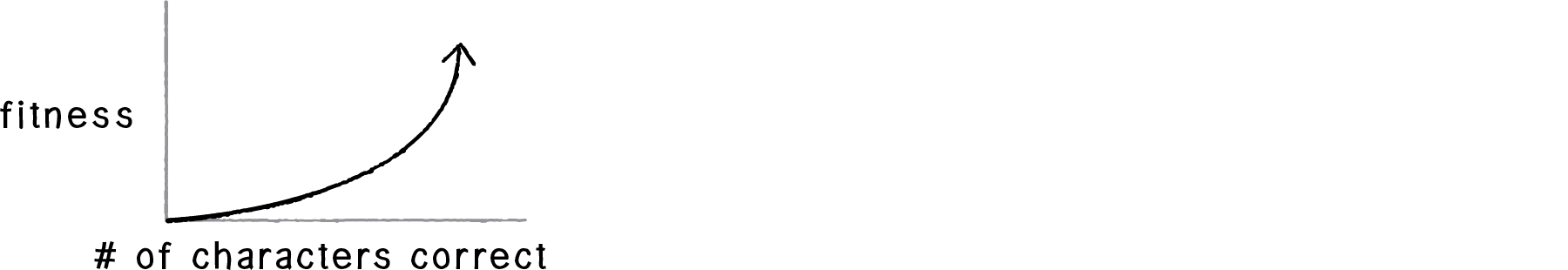
Figure 9.9
The more correct characters, the even greater the fitness. We can achieve this type of result in a number of different ways. For example, we could say:
fitness = (number of correct characters) * (number of correct characters)
Let’s say we have two members of the population, one with five correct characters and one with six. The number 6 is a 20% increase over the number 5. Let’s look at the fitness scores squared.
| Characters correct | Fitness |
|---|---|
5 |
25 |
6 |
36 |
The fitness scores increase exponentially relative to the number of correct characters. 36 is a 44% increase over 25.
Here’s another formula.
fitness = 2(number of correct characters)
| Characters correct | Fitness |
|---|---|
1 |
2 |
2 |
4 |
3 |
8 |
4 |
16 |
Here, the fitness scores increase at a faster rate, doubling with each additional correct character.
Exercise 9.7
Rewrite the fitness function to increase exponentially according to the number of correct characters. Note that you will also have to normalize the fitness values to a range between 0 and 1 so they can be added to the mating pool a reasonable number of times.
While this rather specific discussion of exponential vs. linear fitness functions is an important detail in the design of a good fitness function, I don’t want us to miss the more important point here: Design your own fitness function! I seriously doubt that any project you undertake in Processing with genetic algorithms will actually involve counting the correct number of characters in a string. In the context of this book, it’s more likely you will be looking to evolve a creature that is part of a physics system. Perhaps you are looking to optimize the weights of steering behaviors so a creature can best escape a predator or avoid an obstacle or make it through a maze. You have to ask yourself what you’re hoping to evaluate.
Let’s consider a racing simulation in which a vehicle is evolving a design optimized for speed.
fitness = total number of frames required for vehicle to reach target
How about a cannon that is evolving the optimal way to shoot a target?
fitness = cannonball distance to target
The design of computer-controlled players in a game is also a common scenario. Let’s say you are programming a soccer game in which the user is the goalie. The rest of the players are controlled by your program and have a set of parameters that determine how they kick a ball towards the goal. What would the fitness score for any given player be?
fitness = total goals scored
This, obviously, is a simplistic take on the game of soccer, but it illustrates the point. The more goals a player scores, the higher its fitness, and the more likely its genetic information will appear in the next game. Even with a fitness function as simple as the one described here, this scenario is demonstrating something very powerful—the adaptability of a system. If the players continue to evolve from game to game to game, when a new human user enters the game with a completely different strategy, the system will quickly discover that the fitness scores are going down and evolve a new optimal strategy. It will adapt. (Don’t worry, there is very little danger in this resulting in sentient robots that will enslave all humans.)
In the end, if you do not have a fitness function that effectively evaluates the performance of the individual elements of your population, you will not have any evolution. And the fitness function from one example will likely not apply to a totally different project. So this is the part where you get to shine. You have to design a function, sometimes from scratch, that works for your particular project. And where do you do this? All you have to edit are those few lines of code inside the function that computes the fitness variable.
void fitness() {
  ????????????
  ????????????
  fitness = ??????????
}
Key #3: Genotype and Phenotype
The final key to designing your own genetic algorithm relates to how you choose to encode the properties of your system. What are you trying to express, and how can you translate that expression into a bunch of numbers? What is the genotype and phenotype?
When talking about the fitness function, we happily assumed we could create computer-controlled kickers that each had a “set of parameters that determine how they kick a ball towards the goal.” However, what those parameters are and how you choose to encode them is up to you.
We started with the Shakespeare example because of how easy it was to design both the genotype (an array of characters) and its expression, the phenotype (the string drawn in the window).
The good news is—and we hinted at this at the start of this chapter—you’ve really been doing this all along. Anytime you write a class in Processing, you make a whole bunch of variables.
class Vehicle {
  float maxspeed;
  float maxforce;
  float size;
  float separationWeight;
  // etc.
All we need to do to evolve those parameters is to turn them into an array, so that the array can be used with all of the functions—crossover(), mutate(), etc.—found in the DNA class. One common solution is to use an array of floating point numbers between 0 and 1.
class DNA {
  float[] genes;

  DNA(int num) {
    genes = new float[num];
    for (int i = 0; i < genes.length; i++) {
      genes[i] = float(1);
    }
  }
Notice how we’ve now put the genetic data (genotype) and its expression (phenotype) into two separate classes. The DNA class is the genotype and the Vehicle class uses a DNA object to drive its behaviors and express that data visually—it is the phenotype. The two can be linked by creating a DNA instance inside the Vehicle class itself.
class Vehicle { DNA dna;
float maxspeed;
float maxforce;
float size;
float separationWeight;
  Vehicle() {
    DNA = new DNA(4);
    maxspeed = dna.genes[0];
    maxforce = dna.genes[1];
    size = dna.genes[2];
    separationWeight = dna.genes[3];
}Of course, you most likely don’t want all your variables to have a range between 0 and 1. But rather than try to remember how to adjust those ranges in the DNA class itself, it’s easier to pull the genetic information from the DNA object and use Processing’s map() function to change the range. For example, if you want a size variable between 10 and 72, you would say:
size = map(dna.genes[2],0,1,10,72);In other cases, you will want to design a genotype that is an array of objects. Consider the design of a rocket with a series of “thruster” engines. You could describe each thruster with a PVector that outlines its direction and relative strength.
class DNA {
  PVector[] genes;

  DNA(int num) {
    genes = new float[num];
    for (int i = 0; i < genes.length; i++) {
genes[i] = PVector.random2D(); genes[i].mult(random(10));
}
}
The phenotype would be a Rocket class that participates in a physics system.
class Rocket {
  DNA dna;
  // etc.
What’s great about this technique of dividing the genotype and phenotype into separate classes (DNA and Rocket for example) is that when it comes time to build all of the code, you’ll notice that the DNA class we developed earlier remains intact. The only thing that changes is the array’s data type (float, PVector, etc.) and the expression of that data in the phenotype class.
In the next section, we’ll follow this idea a bit further and walk through the necessary steps for an example that involves moving bodies and an array of PVectors as DNA.
9.10 Evolving Forces: Smart Rockets
We picked the rocket idea for a specific reason. In 2009, Jer Thorp released a genetic algorithms example on his blog entitled “Smart Rockets.” Jer points out that NASA uses evolutionary computing techniques to solve all sorts of problems, from satellite antenna design to rocket firing patterns. This inspired him to create a Flash demonstration of evolving rockets. Here is a description of the scenario:
A population of rockets launches from the bottom of the screen with the goal of hitting a target at the top of the screen (with obstacles blocking a straight line path).
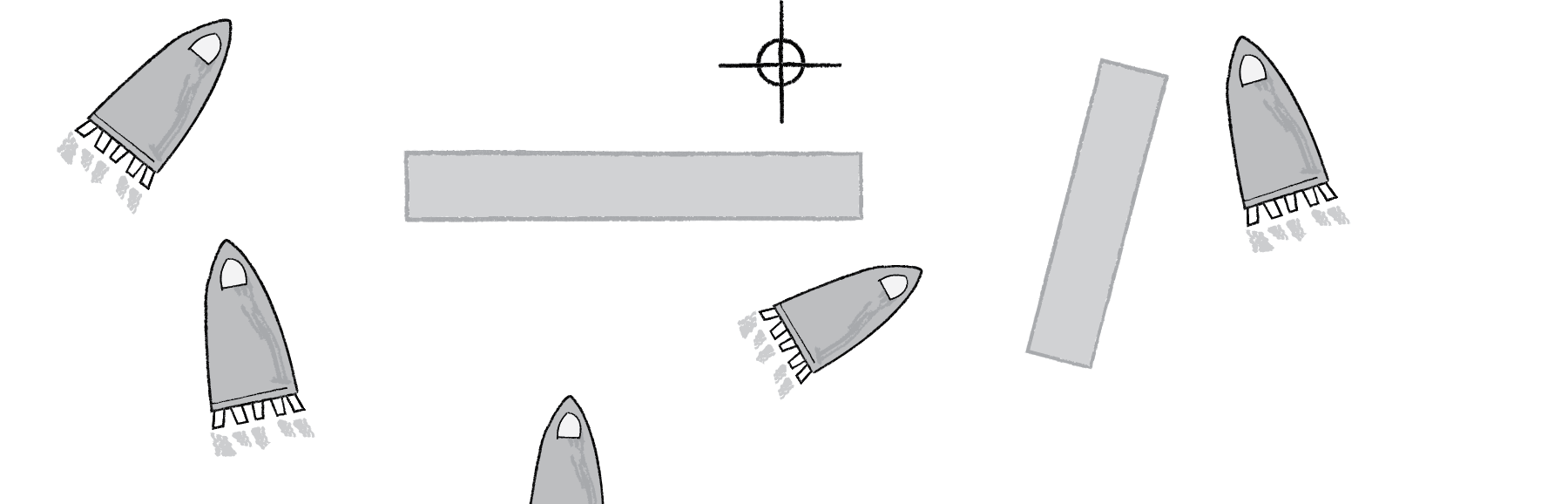
Figure 9.10
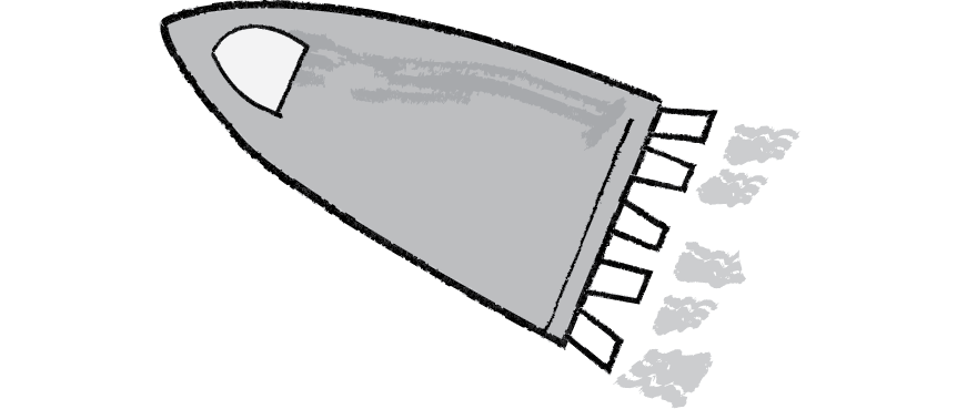
Figure 9.11
Each rocket is equipped with five thrusters of variable strength and direction. The thrusters don’t fire all at once and continuously; rather, they fire one at a time in a custom sequence.
In this section, we’re going to evolve our own simplified Smart Rockets, inspired by Jer Thorp’s. When we get to the end of the section, we’ll leave implementing some of Jer’s additional advanced features as an exercise.
Our rockets will have only one thruster, and this thruster will be able to fire in any direction with any strength for every frame of animation. This isn’t particularly realistic, but it will make building out the framework a little easier. (We can always make the rocket and its thrusters more advanced and realistic later.)
Let’s start by taking our basic Mover class from Chapter 2 examples and renaming it Rocket.
class Rocket {
  PVector location;
  PVector velocity;
  PVector acceleration;
  void applyForce(PVector f) {
    acceleration.add(f);
  }
void update() { velocity.add(acceleration); location.add(velocity);
acceleration.mult(0);
}
}
Using the above framework, we can implement our smart rocket by saying that for every frame of animation, we call applyForce() with a new force. The “thruster” applies a single force to the rocket each time through draw().
Considering this example, let’s go through the three keys to programming our own custom genetic algorithm example as outlined in the previous section.
Key #1: Population size and mutation rate
We can actually hold off on this first key for the moment. Our strategy will be to pick some reasonable numbers (a population of 100 rockets, mutation rate of 1%) and build out the system, playing with these numbers once we have our sketch up and running.
Key #2: The fitness function
We stated the goal of a rocket reaching a target. In other words, the closer a rocket gets to the target, the higher the fitness. Fitness is inversely proportional to distance: the smaller the distance, the greater the fitness; the greater the distance, the smaller the fitness.
Let’s assume we have a PVector target.
void fitness() { float d = PVector.dist(location,target); fitness = 1/d;
}
This is perhaps the simplest fitness function we could write. By using one divided by distance, large distances become small numbers and small distances become large.
| distance | 1 / distance |
|---|---|
300 |
1 / 300 = 0.0033 |
100 |
1 / 100 = 0.01 |
5 |
1 / 5 = 0.2 |
1 |
1 / 1 = 1.0 |
0.1 |
1 / 0.1 = 10 |
And if we wanted to use our exponential trick from the previous section, we could use one divided by distance squared.
| distance | 1 / distance | (1 / distance)2 |
|---|---|---|
300 |
1 / 400 = 0.0025 |
0.00000625 |
100 |
1 / 100 = 0.01 |
0.0001 |
5 |
1 / 5 = 0.2 |
0.04 |
1 |
1 / 1 = 1.0 |
1.0 |
0.1 |
1 / 0.1 = 10 |
100 |
There are several additional improvements we’ll want to make to the fitness function, but this simple one is a good start.
void fitness() {
float d = PVector.dist(location,target);
  fitness = pow(1/d,2);
}
Key #3: Genotype and Phenotype
We stated that each rocket has a thruster that fires in a variable direction with a variable magnitude in each frame. And so we need a PVector for each frame of animation. Our genotype, the data required to encode the rocket’s behavior, is therefore an array of PVectors.
class DNA {
  PVector[] genes;
The happy news here is that we don’t really have to do anything else to the DNA class. All of the functionality we developed for the typing monkey (crossover and mutation) applies here. The one difference we do have to consider is how we initialize the array of genes. With the typing monkey, we had an array of characters and picked a random character for each element of the array. Here we’ll do exactly the same thing and initialize a DNA sequence as an array of random PVectors. Now, your instinct in creating a random PVector might be as follows:
PVector v = new PVector(random(-1,1),random(-1,1));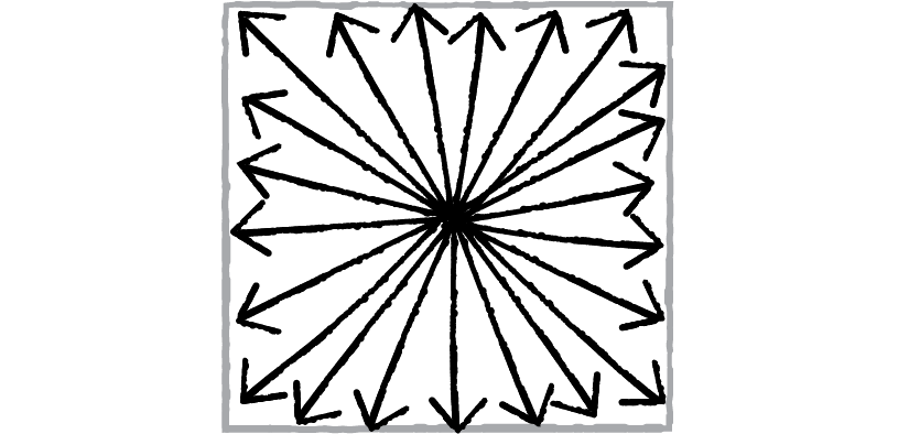
Figure 9.12
This is perfectly fine and will likely do the trick. However, if we were to draw every single possible vector we might pick, the result would fill a square (see Figure 9.12). In this case, it probably doesn’t matter, but there is a slight bias to diagonals here given that a PVector from the center of a square to a corner is longer than a purely vertical or horizontal one.

Figure 9.13
What would be better here is to pick a random angle and make a PVector of length one from that angle, giving us a circle (see Figure 9.13). This could be easily done with a quick polar to Cartesian conversion, but a quicker path to the result is just to use PVector's random2D().
for (int i = 0; i < genes.length; i++) { genes[i] = PVector.random2D();
}
A PVector of length one is actually going to be quite a large force. Remember, forces are applied to acceleration, which accumulates into velocity thirty times per second. So, for this example, we can also add one more variable to the DNA class: a maximum force that scales all the PVectors. This will control the thruster power.
class DNA {
PVector[] genes;
  float maxforce = 0.1;

  DNA() {
    genes = new PVector[lifetime];
    for (int i = 0; i < genes.length; i++) {
      genes[i] = PVector.random2D();
      genes[i].mult(random(0, maxforce));
    }
  }
Notice also that we created an array of PVectors with length lifetime. We need a PVector for each frame of the rocket’s life, and the above assumes the existence of a global variable lifetime that stores the total number of frames in each generation’s life cycle.
The expression of this array of PVectors, the phenotype, is a Rocket class modeled on our basic PVector and forces examples from Chapter 2. All we need to do is add an instance of a DNA object to the class. The fitness variable will also live here. Only the Rocket object knows how to compute its distance to the target, and therefore the fitness function will live here in the phenotype as well.
class Rocket {
DNA dna; float fitness;
PVector location;
PVector velocity;
PVector acceleration;
What are we using the DNA for? We are marching through the array of PVectors and applying them one at a time as a force to the rocket. To do this, we’ll also have to add an integer that acts as a counter to walk through the array.
  int geneCounter = 0;

  void run() {
applyForce(dna.genes[geneCounter]); geneCounter++; update();
}
9.11 Smart Rockets: Putting It All Together
We now have our DNA class (genotype) and our Rocket class (phenotype). The last piece of the puzzle is a Population class, which manages an array of rockets and has the functionality for selection and reproduction. Again, the happy news here is that we barely have to change anything from the Shakespeare monkey example. The process for building a mating pool and generating a new array of child rockets is exactly the same as what we did with our population of strings.
class Population {
  float mutationRate;
  Rocket[] population;
  ArrayList<Rocket> matingPool;
  int generations;
  void fitness() {}
  void selection() {}
  void reproduction() {}
There is one fairly significant change, however. With typing monkeys, a random phrase was evaluated as soon as it was created. The string of characters had no lifespan; it existed purely for the purpose of calculating its fitness and then we moved on. The rockets, however, need to live for a period of time before they can be evaluated; they need to be given a chance to make their attempt at reaching the target. Therefore, we need to add one more function to the Population class that runs the physics simulation itself. This is identical to what we did in the run() function of a particle system—update all the particle locations and draw them.
  void live () {
    for (int i = 0; i < population.length; i++) {
      population[i].run();
    }
  }
Finally, we’re ready for setup() and draw(). Here in the main tab, our primary responsibility is to implement the steps of the genetic algorithm in the appropriate order by calling the functions in the Population class.
    population.fitness();
    population.selection();
    population.reproduction();
However, unlike the Shakespeare example, we don’t want to do this every frame. Rather, our steps work as follows:
Create a population of rockets
Let the rockets live for N frames
Evolve the next generation
Selection
Reproduction
Return to Step #2
Example 9.2: Simple Smart Rockets
int lifetime;
int lifeCounter;
Population population;

void setup() {
  size(640, 480);
  lifetime = 500;
  lifeCounter = 0;

  float mutationRate = 0.01;
  population = new Population(mutationRate, 50);
}

void draw() {
  background(255);
if (lifeCounter < lifetime) { population.live();
lifeCounter++;
} else {
    lifeCounter = 0;
    population.fitness();
    population.selection();
    population.reproduction();
  }
}
The above example works, but it isn’t particularly interesting. After all, the rockets simply evolve to having DNA with a bunch of vectors that point straight upwards. In the next example, we’re going to talk through two suggested improvements for the example and provide code snippets that implement these improvements.
Improvement #1: Obstacles
Adding obstacles that the rockets must avoid will make the system more complex and demonstrate the power of the evolutionary algorithm more effectively. We can make rectangular, stationary obstacles fairly easily by creating a class that stores a location and dimensions.
class Obstacle {
  PVector location;
  float w,h;
We can also write a contains() function that will return true or return false to determine if a rocket has hit the obstacle.
  boolean contains(PVector v) {
    if (v.x > location.x && v.x < location.x + w && v.y > location.y && v.y < location.y + h) {
      return true;
    } else {
      return false;
    }
  }
Assuming we make an ArrayList of obstacles, we can then have each rocket check to see if it has collided with an obstacle and set a boolean flag to be true if it does, adding a function to the rocket class.
  void obstacles() {
    for (Obstacle obs : obstacles) {
      if (obs.contains(location)) {
        stopped = true;
      }
    }
  }
If the rocket hits an obstacle, we choose to stop it from updating its location.
void run() { if (!stopped) {
applyForce(dna.genes[geneCounter]);
geneCounter = (geneCounter + 1) % dna.genes.length;
update();
obstacles();
}
}
And we also have an opportunity to adjust the rocket’s fitness. We consider it to be pretty terrible if the rocket hits an obstacle, and so its fitness should be greatly reduced.
  void fitness() {
    float d = dist(location.x, location.y, target.location.x, target.location.y);
    fitness = pow(1/d, 2);
    if (stopped) fitness *= 0.1;
  }
Improvement #2: Evolve reaching the target faster
If you look closely at our first Smart Rockets example, you’ll notice that the rockets are not rewarded for getting to the target faster. The only variable in their fitness calculation is the distance to the target at the end of the generation’s life. In fact, in the event that the rockets get very close to the target but overshoot it and fly past, they may actually be penalized for getting to the target faster. Slow and steady wins the race in this case.
We could improve the algorithm to optimize for speed a number of ways. First, instead of using the distance to the target at the end of the generation, we could use the distance that is the closest to the target at any point during the rocket’s life. We would call this the rocket’s “record” distance. (All of the code snippets in this section live inside the Rocket class.)
  void checkTarget() {
    float d = dist(location.x, location.y, target.location.x, target.location.y);
if (d < recordDist) recordDist = d;In addition, a rocket should be rewarded according to how quickly it reaches the target. The faster it reaches the target, the higher the fitness. The slower, the lower. To accomplish this, we can increment a counter every cycle of the rocket’s life until it reaches the target. At the end of its life, the counter will equal the amount of time the rocket took to reach that target.
    if (target.contains(location)) {
      hitTarget = true;
    } else if (!hitTarget) {
      finishTime++;
    }
}
Fitness is also inversely proportional to finishTime, and so we can improve our fitness function as follows:
void fitness() {
fitness = (1/(finishTime*recordDist)); fitness = pow(fitness, 2);
if (stopped) fitness *= 0.1; if (hitTarget) fitness *= 2;
}
These improvements are both incorporated into the code for Example 9.3: Smart Rockets.
Exercise 9.8
Create a more complex obstacle course. As you make it more difficult for the rockets to reach the target, do you need to improve other aspects of the GA—for example, the fitness function?
Exercise 9.9
Implement the rocket firing pattern of Jer Thorp’s Smart Rockets. Each rocket only gets five thrusters (of any direction and strength) that follow a firing sequence (of arbitrary length). Jer’s simulation also gives the rockets a finite amount of fuel.
Exercise 9.10
Visualize the rockets differently. Can you draw a line for the shortest path to the target? Can you add particle systems that act as smoke in the direction of the rocket thrusters?
Exercise 9.11
Another way to achieve a similar result is to evolve a flow field. Can you make the genotype of a rocket a flow field of PVectors?
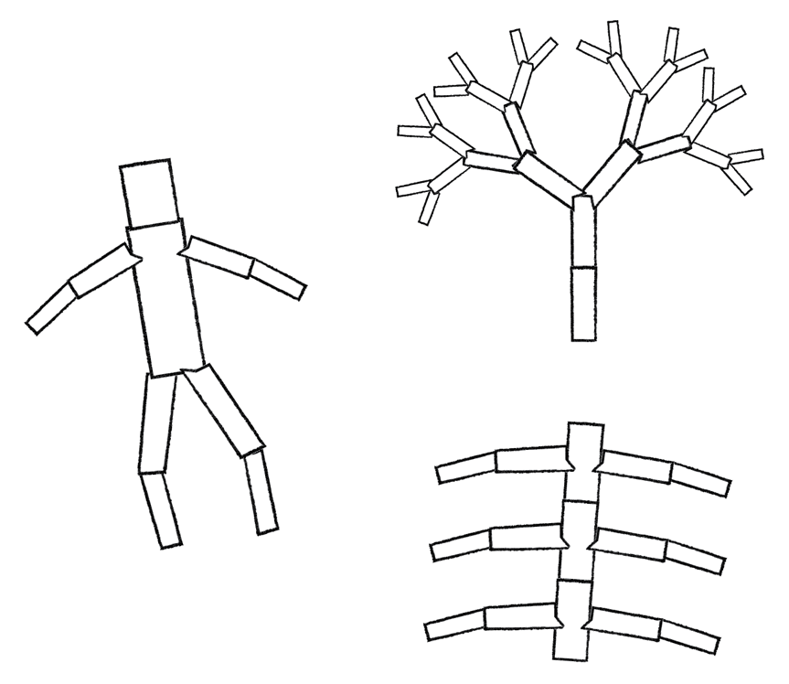
One of the more famous implementations of genetic algorithms in computer graphics is Karl Sims’s “Evolved Virtual Creatures.” In Sims’s work, a population of digital creatures (in a simulated physics environment) is evaluated for the creatures' ability to perform tasks, such as swimming, running, jumping, following, and competing for a green cube.
One of the innovations in Sims’s work is a node-based genotype. In other words, the creature’s DNA is not a linear list of PVectors or numbers, but a map of nodes. (For an example of this, take a look at Exercise 5.15, toxiclibs' Force Directed Graph.) The phenotype is the creature’s design itself, a network of limbs connected with muscles.
Exercise 9.12
Using toxiclibs or Box2D as the physics model, can you create a simplified 2D version of Sims’s creatures? For a lengthier description of Sims’s techniques, I suggest you watch the video and read Sims’s paper Virtual Creatures. In addition, you can find a similar example that uses Box2D to evolve a “car”: BoxCar2D.

9.12 Interactive Selection
In addition to Evolved Virtual Creatures, Sims is also well known for his museum installation Galapagos. Originally installed in the Intercommunication Center in Tokyo in 1997, the installation consists of twelve monitors displaying computer-generated images. These images evolve over time, following the genetic algorithm steps of selection and reproduction. The innovation here is not the use of the genetic algorithm itself, but rather the strategy behind the fitness function. In front of each monitor is a sensor on the floor that can detect the presence of a user viewing the screen. The fitness of an image is tied to the length of time that viewers look at the image. This is known as interactive selection, a genetic algorithm with fitness values assigned by users.
Think of all the rating systems you’ve ever used. Could you evolve the perfect movie by scoring all films according to your Netflix ratings? The perfect singer according to American Idol voting?
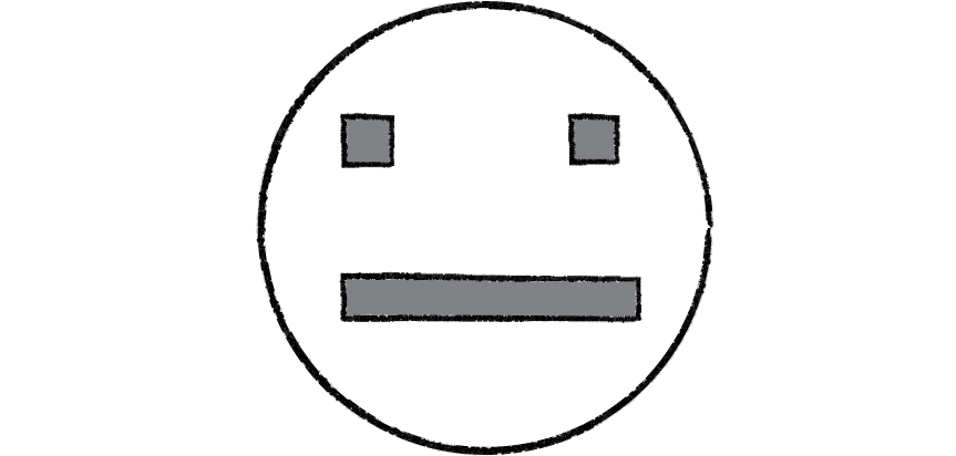
Figure 9.14
To illustrate this technique, we’re going to build a population of simple faces. Each face will have a set of properties: head size, head color, eye location, eye size, mouth color, mouth location, mouth width, and mouth height.
The face’s DNA (genotype) is an array of floating point numbers between 0 and 1, with a single value for each property.
class DNA {

  float[] genes;
  int len = 20;

  DNA() {
    genes = new float[len];
    for (int i = 0; i < genes.length; i++) {
      genes[i] = random(0,1);
    }
  }
The phenotype is a Face class that includes an instance of a DNA object.
class Face {

  DNA dna;
  float fitness;
When it comes time to draw the face on screen, we can use Processing’s map() function to convert any gene value to the appropriate range for pixel dimensions or color values. (In this case, we are also using colorMode() to set the RGB ranges between 0 and 1.)
void display() { float r = map(dna.genes[0],0,1,0,70);
color c = color(dna.genes[1],dna.genes[2],dna.genes[3]);
float eye_y = map(dna.genes[4],0,1,0,5);
float eye_x = map(dna.genes[5],0,1,0,10);
float eye_size = map(dna.genes[5],0,1,0,10);
color eyecolor = color(dna.genes[4],dna.genes[5],dna.genes[6]);
color mouthColor = color(dna.genes[7],dna.genes[8],dna.genes[9]);
float mouth_y = map(dna.genes[5],0,1,0,25);
float mouth_x = map(dna.genes[5],0,1,-25,25);
float mouthw = map(dna.genes[5],0,1,0,50);
float mouthh = map(dna.genes[5],0,1,0,10);
So far, we’re not really doing anything new. This is what we’ve done in every GA example so far. What’s new is that we are not going to write a fitness() function in which the score is computed based on a math formula. Instead, we are going to ask the user to assign the fitness.
Now, how best to ask a user to assign fitness is really more of an interaction design problem, and it isn’t really within the scope of this book. So we’re not going to launch into an elaborate discussion of how to program sliders or build your own hardware dials or build a Web app for users to submit online scores. How you choose to acquire fitness scores is really up to you and the particular application you are developing.
For this simple demonstration, we’ll increase fitness whenever a user rolls the mouse over a face. The next generation is created when the user presses a button with an “evolve next generation” label.
Let’s look at how the steps of the genetic algorithm are applied in the main tab, noting how fitness is assigned according to mouse interaction and the next generation is created on a button press. The rest of the code for checking mouse locations, button interactions, etc. can be found in the accompanying example code.
Example 9.4: Interactive selection
Population population;
Button button;

void setup() {
  size(780,200);
  float mutationRate = 0.05;
  population = new Population(mutationRate,10);
  button = new Button(15,150,160,20, "evolve new generation");
}

void draw() {

  population.display();
  population.rollover(mouseX,mouseY);
  button.display();
}

void mousePressed() {
  if (button.clicked(mouseX,mouseY)) {
    population.selection();
    population.reproduction();
  }
}
This example, it should be noted, is really just a demonstration of the idea of interactive selection and does not achieve a particularly meaningful result. For one, we didn’t take much care in the visual design of the faces; they are just a few simple shapes with sizes and colors. Sims, for example, used more elaborate mathematical functions as his images’ genotype. You might also consider a vector-based approach, in which a design’s genotype is a set of points and/or paths.
The more significant problem here, however, is one of time. In the natural world, evolution occurs over millions of years. In the computer simulation world of our previous examples, we were able to evolve behaviors relatively quickly because we were producing new generations algorithmically. In the Shakespeare monkey example, a new generation was born in each frame of animation (approximately sixty per second). Since the fitness values were computed according to a math formula, we could also have had arbitrarily large populations that increased the speed of evolution. In the case of interactive selection, however, we have to sit and wait for a user to rate each and every member of the population before we can get to the next generation. A large population would be unreasonably tedious to deal with—not to mention, how many generations could you stand to sit through?
There are certainly clever solutions around this. Sims’s Galapagos exhibit concealed the rating process from the users, as it occurred through the normal behavior of looking at artwork in a museum setting. Building a Web application that would allow many users to rate a population in a distributed fashion is also a good strategy for achieving many ratings for large populations quickly.
In the end, the key to a successful interactive selection system boils down to the same keys we previously established. What is the genotype and phenotype? And how do you calculate fitness, which in this case we can revise to say: “What is your strategy for assigning fitness according to user interaction?”
9.13 Ecosystem Simulation
You may have noticed something a bit odd about every single evolutionary system we’ve built so far in this chapter. After all, in the real world, a population of babies isn’t born all at the same time. Those babies don’t then grow up and all reproduce at exactly the same time, then instantly die to leave the population size perfectly stable. That would be ridiculous. Not to mention the fact that there is certainly no one running around the forest with a calculator crunching numbers and assigning fitness values to all the creatures.
In the real world, we don’t really have “survival of the fittest”; we have “survival of the survivors.” Things that happen to live longer, for whatever reason, have a greater chance of reproducing. Babies are born, they live for a while, maybe they themselves have babies, maybe they don’t, and then they die.
You won’t necessarily find simulations of “real-world” evolution in artificial intelligence textbooks. Genetic algorithms are generally used in the more formal manner we outlined in this chapter. However, since we are reading this book to develop simulations of natural systems, it’s worth looking at some ways in which we might use a genetic algorithm to build something that resembles a living “ecosystem,” much like the one we’ve described in the exercises at the end of each chapter.
Let’s begin by developing a very simple scenario. We’ll create a creature called a "bloop," a circle that moves about the screen according to Perlin noise. The creature will have a radius and a maximum speed. The bigger it is, the slower it moves; the smaller, the faster.
class Bloop { PVector location;
  float r;
  float maxspeed;
  float xoff, yoff;

  void update() {
    float vx = map(noise(xoff),0,1,-maxspeed,maxspeed);
    float vy = map(noise(yoff),0,1,-maxspeed,maxspeed);
    PVector velocity = new PVector(vx,vy);
    xoff += 0.01;
    yoff += 0.01;
    location.add(velocity);
  }
  void display() {
    ellipse(location.x, location.y, r, r);
  }
}
The above is missing a few details (such as initializing the variables in the constructor), but you get the idea.
For this example, we’ll want to store the population of bloops in an ArrayList, rather than an array, as we expect the population to grow and shrink according to how often bloops die or are born. We can store this ArrayList in a class called World, which will manage all the elements of the bloops’ world.
class World {
  ArrayList<Bloop> bloops;

  World(int num) {
    bloops = new ArrayList<Bloop>();

    for (int i = 0; i < num; i++) {
      bloops.add(new Bloop());
    }
  }
So far, what we have is just a rehashing of our particle system example from Chapter 5. We have an entity (Bloop) that moves around the window and a class (World) that manages a variable quantity of these entities. To turn this into a system that evolves, we need to add two additional features to our world:
Bloops die.
Bloops are born.
Bloops dying is our replacement for a fitness function, the process of “selection.” If a bloop dies, it cannot be selected to be a parent, because it simply no longer exists! One way we can build a mechanism to ensure bloop deaths in our world is by adding a health variable to the Bloop class.
class Bloop { float health = 100;In each frame of animation, a bloop loses some health.
void update() { health -= 1;
}
If health drops below 0, the bloop dies.
  boolean dead() {
    if (health < 0.0) {
      return true;
    } else {
      return false;
    }
  }
This is a good first step, but we haven’t really achieved anything. After all, if all bloops start with 100 health points and lose 1 point per frame, then all bloops will live for the exact same amount of time and die together. If every single bloop lives the same amount of time, they all have equal chances of reproducing and therefore nothing will evolve.
There are many ways we could achieve variable lifespans with a more sophisticated world. For example, we could introduce predators that eat bloops. Perhaps the faster bloops would be able to escape being eaten more easily, and therefore our world would evolve to have faster and faster bloops. Another option would be to introduce food. When a bloop eats food, it increases its health points, and therefore extends its life.
Let’s assume we have an ArrayList of PVector locations for food, named “food.” We could test each bloop’s proximity to each food location. If the bloop is close enough, it eats the food (which is then removed from the world) and increases its health.
  void eat() {
    for (int i = food.size()-1; i >= 0; i--) {
      PVector foodLocation = food.get(i);
      float d = PVector.dist(location, foodLocation);
if (d < r/2) {
health += 100; food.remove(i);
}
}
}
Now we have a scenario in which bloops that eat more food live longer and have a greater likelihood of reproducing. Therefore, we expect that our system would evolve bloops with an optimal ability to find and eat food.
Now that we have built our world, it’s time to add the components required for evolution. First we should establish our genotype and phenotype.
Genotype and Phenotype
The ability for a bloop to find food is tied to two variables—size and speed. Bigger bloops will find food more easily simply because their size will allow them to intersect with food locations more often. And faster bloops will find more food because they can cover more ground in a shorter period of time.
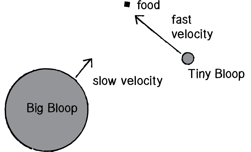
Figure 9.15
Since size and speed are inversely related (large bloops are slow, small bloops are fast), we only need a genotype with a single number.
class DNA {

  float[] genes;

  DNA() {
    genes = new float[1];
    for (int i = 0; i < genes.length; i++) {
      genes[i] = random(0,1);
    }
  }
The phenotype then is the bloop itself, whose size and speed is assigned by adding an instance of a DNA object to the Bloop class.
class Bloop {
  PVector location;
  float health;
  DNA dna;
  float r;
  float maxspeed;

  Bloop(DNA dna_) {
    location = new PVector(width/2,height/2);
    health = 200;
    dna = dna_;
    maxspeed = map(dna.genes[0], 0, 1, 15, 0);
    r        = map(dna.genes[0], 0, 1, 0, 50);
}Notice that with maxspeed, the range is mapped to between 15 and 0, meaning a bloop with a gene value of 0 moves at a speed of 15 and a bloop with a gene value of 1 doesn’t move at all (speed of 0).
Selection and Reproduction
Now that we have the genotype and phenotype, we need to move on to devising a means for bloops to be selected as parents. We stated before that the longer a bloop lives, the more chances it has to reproduce. The length of life is the bloop’s fitness.
One option would be to say that whenever two bloops come into contact with each other, they make a new bloop. The longer a bloop lives, the more likely it is to come into contact with another bloop. (This would also affect the evolutionary outcome given that, in addition to eating food, their ability to find other bloops is a factor in the likelihood of having a baby.)
A simpler option would be to have “asexual” reproduction, meaning a bloop does not require a partner. It can, at any moment, make a clone of itself, another bloop with the same genetic makeup. If we state this selection algorithm as follows:
At any given moment, a bloop has a 1% chance of reproducing.
…then the longer a bloop lives, the more likely it will make at least one child. This is equivalent to saying the more times you play the lottery, the greater the likelihood you’ll win (though I’m sorry to say your chances of that are still essentially zero).
To implement this selection algorithm, we can write a function in the Bloop class that picks a random number every frame. If the number is less than 0.01 (1%), a new bloop is born.
Bloop reproduce() {
    if (random(1) < 0.01) {
       // Make the Bloop baby
    }
  }
How does a bloop reproduce? In our previous examples, the reproduction process involved calling the crossover() function in the DNA class and making a new object from the newly made DNA. Here, since we are making a child from a single parent, we’ll call a function called copy() instead.
  Bloop reproduce() {
    if (random(1) < 0.0005) {
DNA childDNA = dna.copy(); childDNA.mutate(0.01); return new Bloop(location, childDNA);
} else {
      return null;
    }
  }
Note also that we’ve reduced the probability of reproducing from 1% to 0.05%. This value makes quite a difference; with a high probability of reproducing, the system will quickly tend towards overpopulation. Too low a probability, and everything will likely quickly die out.
Writing the copy() function into the DNA class is easy since Processing includes a function arraycopy() that copies the contents of one array into another.
class DNA {
DNA copy() {
    float[] newgenes = new float[genes.length];
    arraycopy(genes,newgenes);
    return new DNA(newgenes);
  }
}
Now that we have all the pieces in place for selection and reproduction, we can finalize the World class that manages the list of all Bloop objects (as well as a Food object, which itself is a list of PVector locations for food).
Before you run the example, take a moment to guess what size and speed of bloops the system will evolve towards. We’ll discuss following the code.
Example 9.5: Evolution ecosystem
World world;
void setup() {
  size(600,400);
  world = new World(20);
}

void draw() {
  background(255);
  world.run();
}
class World {
  ArrayList<Bloop> bloops;
  Food food;

  World(int num) {
    food = new Food(num);
    bloops = new ArrayList<Bloop>();
    for (int i = 0; i < num; i++) {
      PVector location = new PVector(random(width),random(height));
      DNA dna = new DNA();
      bloops.add(new Bloop(l,dna));
    }
  }

  void run() {
    food.run();

    for (int i = bloops.size()-1; i >= 0; i--) {
      Bloop b = bloops.get(i);
      b.run();
      b.eat(food);
      if (b.dead()) {
        bloops.remove(i);
        food.add(b.location);
      }
      Bloop child = b.reproduce();
      if (child != null) bloops.add(child);
    }
  }
}
If you guessed medium-sized bloops with medium speed, you were right. With the design of this system, bloops that are large are simply too slow to find food. And bloops that are fast are too small to find food. The ones that are able to live the longest tend to be in the middle, large enough and fast enough to find food (but not too large or too fast). There are also some anomalies. For example, if it so happens that a bunch of large bloops end up in the same location (and barely move because they are so large), they may all die out suddenly, leaving a lot of food for one large bloop who happens to be there to eat and allowing a mini-population of large bloops to sustain themselves for a period of time in one location.
This example is rather simplistic given its single gene and asexual reproduction. Here are some suggestions for how you might apply the bloop example in a more elaborate ecosystem simulation.
The Ecosystem Project
Step 9 Exercise:
Add evolution to your ecosystem, building from the examples in this chapter.
Add a population of predators to your ecosystem. Biological evolution between predators and prey (or parasites and hosts) is often referred to as an “arms race,” in which the creatures continuously adapt and counter-adapt to each other. Can you achieve this behavior in a system of multiple creatures?
How would you implement crossover and mutation between two parents in an ecosystem modeled after the bloops? Try implementing an algorithm so that two creatures meet and mate when within a certain proximity. Can you make creatures with gender?
Try using the weights of multiple steering forces as a creature’s DNA. Can you create a scenario in which creatures evolve to cooperate with each other?
One of the greatest challenges in ecosystem simulations is achieving a nice balance. You will likely find that most of your attempts result in either mass overpopulation (followed by mass extinction) or simply mass extinction straight away. What techniques can you employ to achieve balance? Consider using the genetic algorithm itself to evolve optimal parameters for an ecosystem.

