6.1 Forces from Within

The term autonomous agent generally refers to an entity that makes its own choices about how to act in its environment without any influence from a leader or global plan. For us, “acting” will mean moving. This addition is a significant conceptual leap. Instead of a box sitting on a boundary waiting to be pushed by another falling box, we are now going to design a box that has the ability and “desire” to leap out of the way of that other falling box, if it so chooses. While the concept of forces that come from within is a major shift in our design thinking, our code base will barely change, as these desires and actions are simply that—forces.

Here are three key components of autonomous agents that we’ll want to keep in mind as we build our examples.

In the late 1980s, computer scientist Craig Reynolds developed algorithmic steering behaviors for animated characters. These behaviors allowed individual elements to navigate their digital environments in a “lifelike” manner with strategies for fleeing, wandering, arriving, pursuing, evading, etc. Used in the case of a single autonomous agent, these behaviors are fairly simple to understand and implement. In addition, by building a system of multiple characters that steer themselves according to simple, locally based rules, surprising levels of complexity emerge. The most famous example is Reynolds’s “boids” model for “flocking/swarming” behavior.

6.2 Vehicles and Steering

Now that we understand the core concepts behind autonomous agents, we can begin writing the code. There are many places where we could start. Artificial simulations of ant and termite colonies are fantastic demonstrations of systems of autonomous agents. (For more on this topic, I encourage you to read Turtles, Termites, and Traffic Jams by Mitchel Resnick.) However, we want to begin by examining agent behaviors that build on the work we’ve done in the first five chapters of this book: modeling motion with vectors and driving motion with forces. And so it’s time to rename our Mover class that became our Particle class once again. This time we are going to call it Vehicle.

class Vehicle {
 
  PVector location;
  PVector velocity;
  PVector acceleration;
 
  // What else do we need to add?

In his 1999 paper “Steering Behaviors for Autonomous Characters,” Reynolds uses the word “vehicle” to describe his autonomous agents, so we will follow suit.

Reynolds describes the motion of idealized vehicles (idealized because we are not concerned with the actual engineering of such vehicles, but simply assume that they exist and will respond to our rules) as a series of three layers—Action Selection, Steering, and Locomotion.

Ultimately, the most important layer for you to consider is #1—Action Selection. What are the elements of your system and what are their goals? In this chapter, we are going to look at a series of steering behaviors (i.e. actions): seek, flee, follow a path, follow a flow field, flock with your neighbors, etc. It’s important to realize, however, that the point of understanding how to write the code for these behaviors is not because you should use them in all of your projects. Rather, these are a set of building blocks, a foundation from which you can design and develop vehicles with creative goals and new and exciting behaviors. And even though we will think literally in this chapter (follow that pixel!), you should allow yourself to think more abstractly (like Braitenberg). What would it mean for your vehicle to have “love” or “fear” as its goal, its driving force? Finally (and we’ll address this later in the chapter), you won’t get very far by developing simulations with only one action. Yes, our first example will be “seek a target.” But for you to be creative—to make these steering behaviors your own—it will all come down to mixing and matching multiple actions within the same vehicle. So view these examples not as singular behaviors to be emulated, but as pieces of a larger puzzle that you will eventually assemble.

6.3 The Steering Force

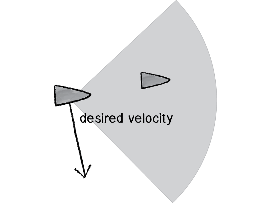
We can entertain ourselves by discussing the theoretical principles behind autonomous agents and steering as much as we like, but we can’t get anywhere without first understanding the concept of a steering force. Consider the following scenario. A vehicle moving with velocity desires to seek a target.

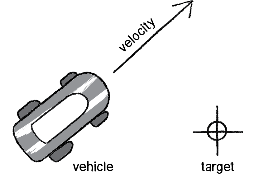
Figure 6.1

Its goal and subsequent action is to seek the target in Figure 6.1. If you think back to Chapter 2, you might begin by making the target an attractor and apply a gravitational force that pulls the vehicle to the target. This would be a perfectly reasonable solution, but conceptually it’s not what we’re looking for here. We don’t want to simply calculate a force that pushes the vehicle towards its target; rather, we are asking the vehicle to make an intelligent decision to steer towards the target based on its perception of its state and environment (i.e. how fast and in what direction is it currently moving). The vehicle should look at how it desires to move (a vector pointing to the target), compare that goal with how quickly it is currently moving (its velocity), and apply a force accordingly.

steering force = desired velocity - current velocity

Or as we might write in Processing:

PVector steer = PVector.sub(desired,velocity);

In the above formula, velocity is no problem. After all, we’ve got a variable for that. However, we don’t have the desired velocity; this is something we have to calculate. Let’s take a look at Figure 6.2. If we’ve defined the vehicle’s goal as “seeking the target,” then its desired velocity is a vector that points from its current location to the target location.

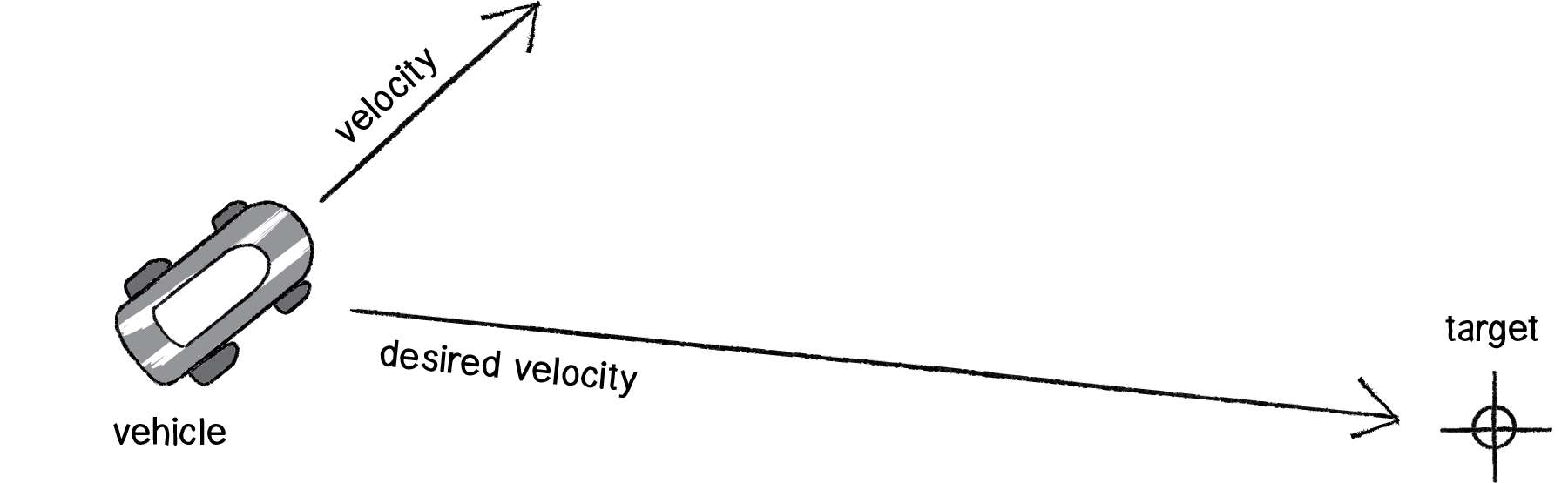
Figure 6.2

Assuming a PVector target, we then have:

PVector desired = PVector.sub(target,location);

But this isn’t particularly realistic. What if we have a very high-resolution window and the target is thousands of pixels away? Sure, the vehicle might desire to teleport itself instantly to the target location with a massive velocity, but this won’t make for an effective animation. What we really want to say is:

The vehicle desires to move towards the target at maximum speed.

In other words, the vector should point from location to target and with a magnitude equal to maximum speed (i.e. the fastest the vehicle can go). So first, we need to make sure we add a variable to our Vehicle class that stores maximum speed.

class Vehicle {
  PVector location;
  PVector velocity;
  PVector acceleration;

  float maxspeed;

Then, in our desired velocity calculation, we scale according to maximum speed.

PVector desired = PVector.sub(target,location);
desired.normalize();
desired.mult(maxspeed);

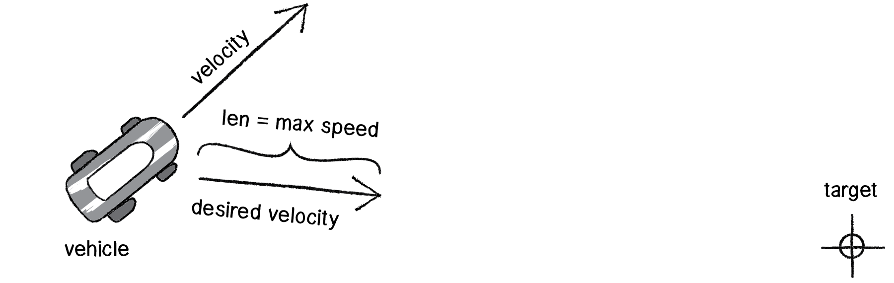
Figure 6.3

Putting this all together, we can write a function called seek() that receives a PVector target and calculates a steering force towards that target.

  void seek(PVector target) {
    PVector desired = PVector.sub(target,location);
    desired.normalize();

    desired.mult(maxspeed);
 

    PVector steer = PVector.sub(desired,velocity);

    applyForce(steer);
  }

Note how in the above function we finish by passing the steering force into applyForce(). This assumes that we are basing this example on the foundation we built in Chapter 2. However, you could just as easily use the steering force with Box2D’s applyForce() function or toxiclibs’ addForce() function.

So why does this all work so well? Let’s see what the steering force looks like relative to the vehicle and target locations.

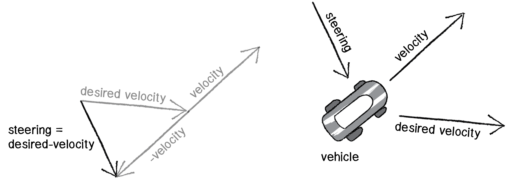
Figure 6.4

Again, notice how this is not at all the same force as gravitational attraction. Remember one of our principles of autonomous agents: An autonomous agent has a limited ability to perceive its environment. Here is that ability, subtly embedded into Reynolds’s steering formula. If the vehicle weren’t moving at all (zero velocity), desired minus velocity would be equal to desired. But this is not the case. The vehicle is aware of its own velocity and its steering force compensates accordingly. This creates a more active simulation, as the way in which the vehicle moves towards the targets depends on the way it is moving in the first place.

In all of this excitement, however, we’ve missed one last step. What sort of vehicle is this? Is it a super sleek race car with amazing handling? Or a giant Mack truck that needs a lot of advance notice to turn? A graceful panda, or a lumbering elephant? Our example code, as it stands, has no feature to account for this variability in steering ability. Steering ability can be controlled by limiting the magnitude of the steering force. Let’s call that limit the “maximum force” (or maxforce for short). And so finally, we have:

class Vehicle {
  PVector location;
  PVector velocity;
  PVector acceleration;

  float maxspeed;

  float maxforce;

followed by:

  void seek(PVector target) {
    PVector desired = PVector.sub(target,location);
    desired.normalize();
    desired.mult(maxspeed);
    PVector steer = PVector.sub(desired,velocity);
 

    steer.limit(maxforce);
 
    applyForce(steer);
  }

Limiting the steering force brings up an important point. We must always remember that it’s not actually our goal to get the vehicle to the target as fast as possible. If that were the case, we would just say “location equals target” and there the vehicle would be. Our goal, as Reynolds puts it, is to move the vehicle in a “lifelike and improvisational manner.” We’re trying to make it appear as if the vehicle is steering its way to the target, and so it’s up to us to play with the forces and variables of the system to simulate a given behavior. For example, a large maximum steering force would result in a very different path than a small one. One is not inherently better or worse than the other; it depends on your desired effect. (And of course, these values need not be fixed and could change based on other conditions. Perhaps a vehicle has health: the higher the health, the better it can steer.)

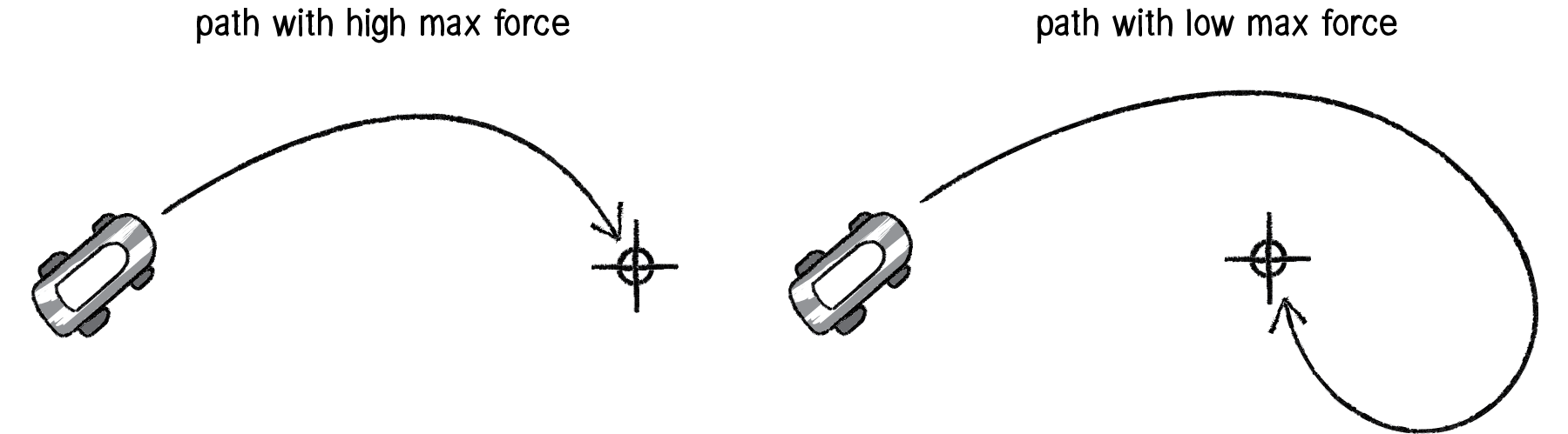
Figure 6.5

Here is the full Vehicle class, incorporating the rest of the elements from the Chapter 2 Mover object.

Example 6.1: Seeking a target

class Vehicle {
 
  PVector location;
  PVector velocity;
  PVector acceleration;

  float r;
  float maxforce;
  float maxspeed;
 
  Vehicle(float x, float y) {
    acceleration = new PVector(0,0);
    velocity = new PVector(0,0);
    location = new PVector(x,y);
    r = 3.0;

    maxspeed = 4;
    maxforce = 0.1;

  }
 

  void update() {
    velocity.add(acceleration);
    velocity.limit(maxspeed);
    location.add(velocity);
    acceleration.mult(0);
  }
 

  void applyForce(PVector force) {
    acceleration.add(force);
  }
 

  void seek(PVector target) {
    PVector desired = PVector.sub(target,location);
    desired.normalize();
    desired.mult(maxspeed);
    PVector steer = PVector.sub(desired,velocity);
    steer.limit(maxforce);
    applyForce(steer);
  }
 
  void display() {

    float theta = velocity.heading() + PI/2;
    fill(175);
    stroke(0);
    pushMatrix();
    translate(location.x,location.y);
    rotate(theta);
    beginShape();
    vertex(0, -r*2);
    vertex(-r, r*2);
    vertex(r, r*2);
    endShape(CLOSE);
    popMatrix();
  }

6.4 Arriving Behavior

After working for a bit with the seeking behavior, you probably are asking yourself, “What if I want my vehicle to slow down as it approaches the target?” Before we can even begin to answer this question, we should look at the reasons behind why the seek behavior causes the vehicle to fly past the target so that it has to turn around and go back. Let’s consider the brain of a seeking vehicle. What is it thinking?

Frame 1: I want to go as fast as possible towards the target!
Frame 2: I want to go as fast as possible towards the target!
Frame 3: I want to go as fast as possible towards the target!
Frame 4: I want to go as fast as possible towards the target!
Frame 5: I want to go as fast as possible towards the target!
etc.

The vehicle is so gosh darn excited about getting to the target that it doesn’t bother to make any intelligent decisions about its speed relative to the target’s proximity. Whether it’s far away or very close, it always wants to go as fast as possible.

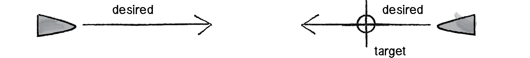
Figure 6.6

In some cases, this is the desired behavior (if a missile is flying at a target, it should always travel at maximum speed.) However, in many other cases (a car pulling into a parking spot, a bee landing on a flower), the vehicle’s thought process needs to consider its speed relative to the distance from its target. For example:

Frame 1: I’m very far away. I want to go as fast as possible towards the target!
Frame 2: I’m very far away. I want to go as fast as possible towards the target!
Frame 3: I’m somewhat far away. I want to go as fast as possible towards the target!
Frame 4: I’m getting close. I want to go more slowly towards the target!
Frame 5: I’m almost there. I want to go very slowly towards the target!
Frame 6: I’m there. I want to stop!

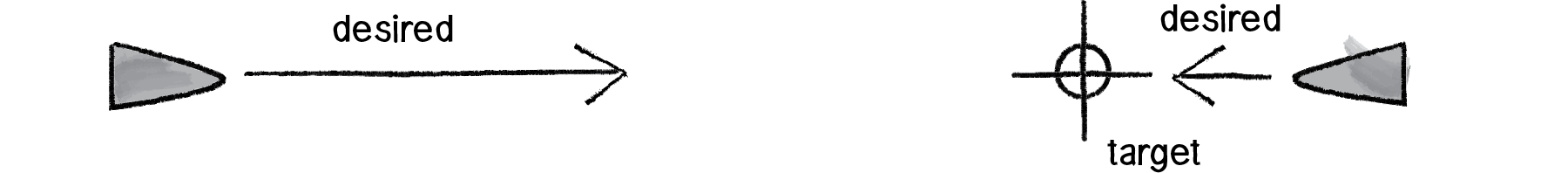
Figure 6.7

How can we implement this “arriving” behavior in code? Let’s return to our seek() function and find the line of code where we set the magnitude of the desired velocity.

   PVector desired = PVector.sub(target,location);
   desired.normalize();
   desired.mult(maxspeed);

In Example 6.1, the magnitude of the desired vector is always “maximum” speed.

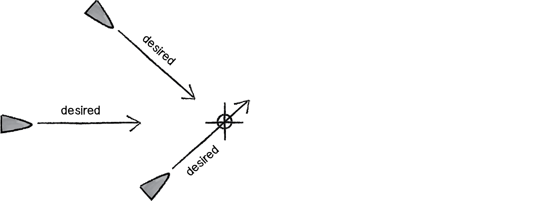
Figure 6.8

What if we instead said the desired velocity is equal to half the distance?

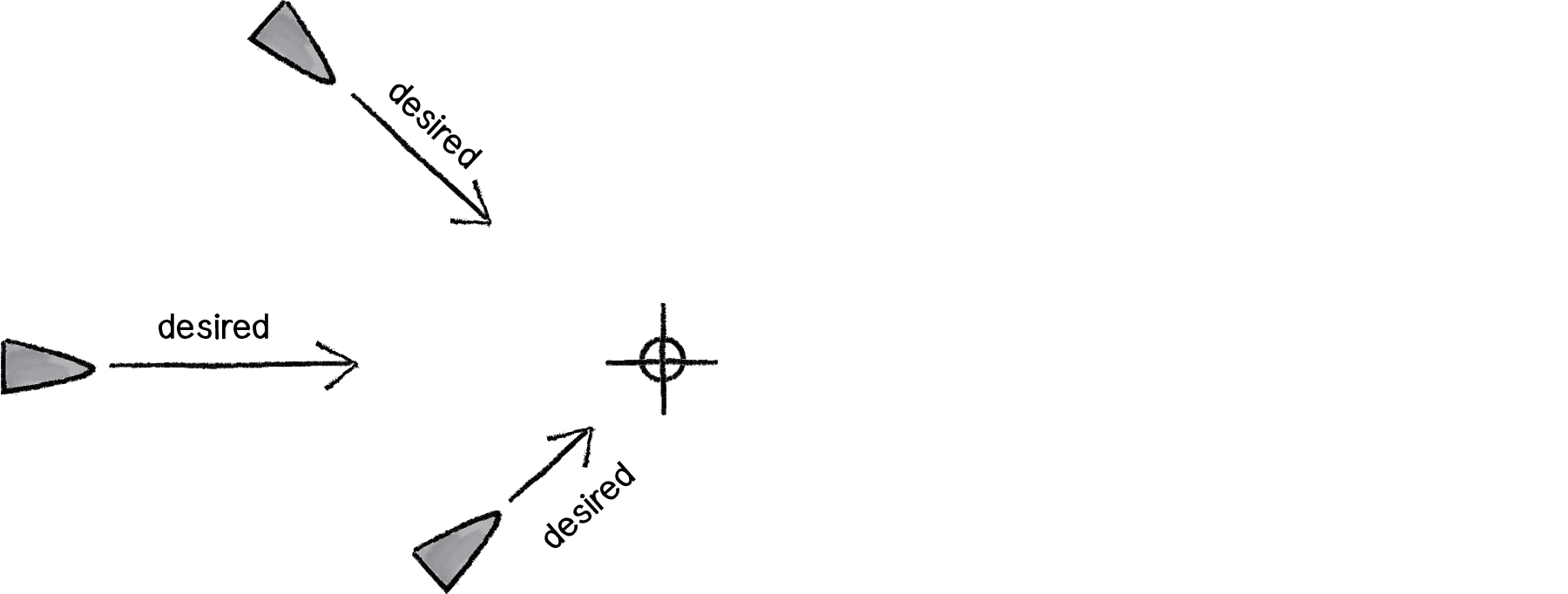
Figure 6.9

   PVector desired = PVector.sub(target,location);
   desired.div(2);

While this nicely demonstrates our goal of a desired speed tied to our distance from the target, it’s not particularly reasonable. After all, 10 pixels away is rather close and a desired speed of 5 is rather large. Something like a desired velocity with a magnitude of 5% of the distance would work much better.

  PVector desired = PVector.sub(target,location);
  desired.mult(0.05);

Reynolds describes a more sophisticated approach. Let’s imagine a circle around the target with a given radius. If the vehicle is within that circle, it slows down—at the edge of the circle, its desired speed is maximum speed, and at the target itself, its desired speed is 0.

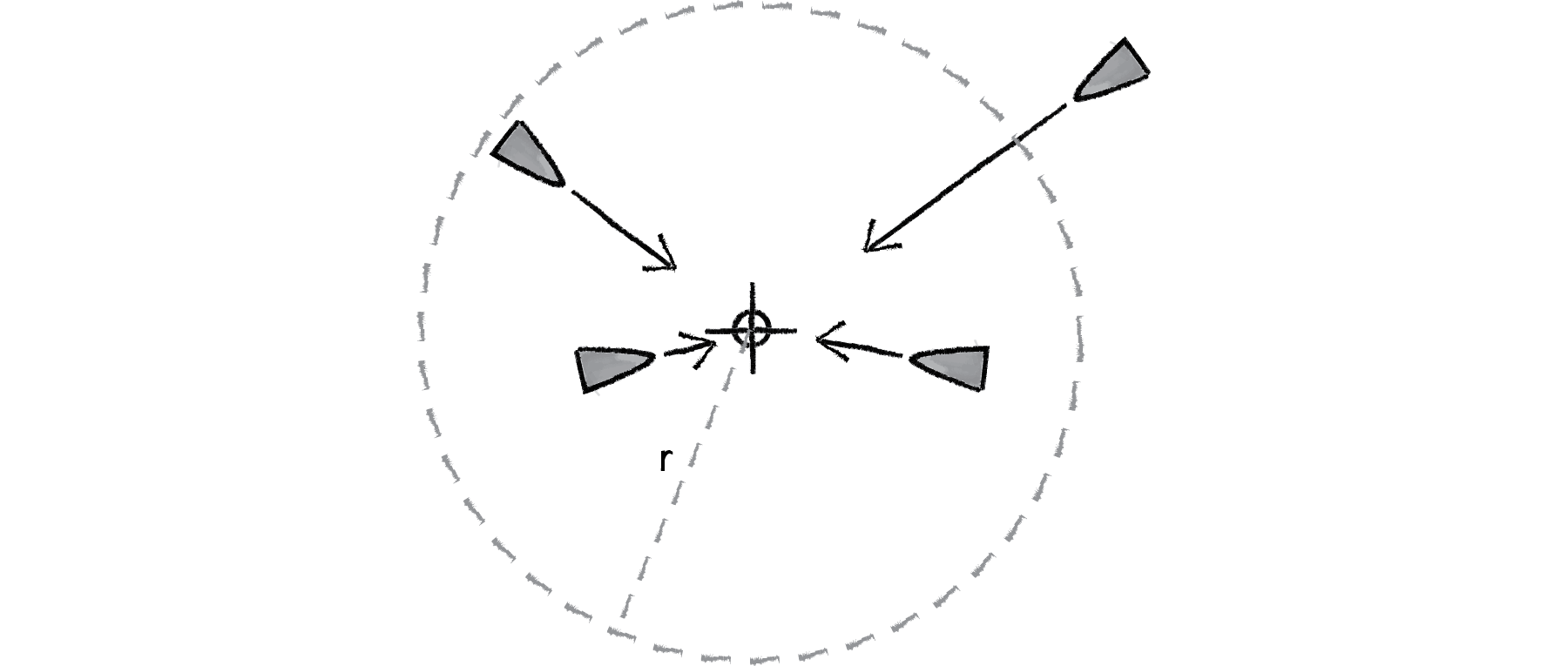
Figure 6.10

In other words, if the distance from the target is less than r, the desired speed is between 0 and maximum speed mapped according to that distance.

Example 6.2: Arrive steering behavior

  void arrive(PVector target) {
    PVector desired = PVector.sub(target,location);
 

    float d = desired.mag();
    desired.normalize();

    if (d < 100) {

      float m = map(d,0,100,0,maxspeed);
      desired.mult(m);

    } else {

      desired.mult(maxspeed);
    }
 

    PVector steer = PVector.sub(desired,velocity);
    steer.limit(maxforce);
    applyForce(steer);
  }

The arrive behavior is a great demonstration of the magic of “desired minus velocity.” Let’s examine this model again relative to how we calculated forces in earlier chapters. In the “gravitational attraction” examples, the force always pointed directly from the object to the target (the exact direction of the desired velocity), whether the force was strong or weak.

The steering function, however, says: “I have the ability to perceive the environment.” The force isn’t based on just the desired velocity, but on the desired velocity relative to the current velocity. Only things that are alive can know their current velocity. A box falling off a table doesn’t know it’s falling. A cheetah chasing its prey, however, knows it is chasing.

The steering force, therefore, is essentially a manifestation of the current velocity’s error: "I’m supposed to be going this fast in this direction, but I’m actually going this fast in another direction. My error is the difference between where I want to go and where I am currently going." Taking that error and applying it as a steering force results in more dynamic, lifelike simulations. With gravitational attraction, you would never have a force pointing away from the target, no matter how close. But with arriving via steering, if you are moving too fast towards the target, the error would actually tell you to slow down!

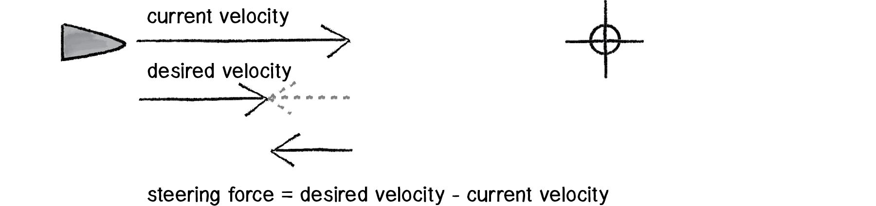
Figure 6.11

6.5 Your Own Desires: Desired Velocity

The first two examples we’ve covered—seek and arrive—boil down to calculating a single vector for each behavior: the desired velocity. And in fact, every single one of Reynolds’s steering behaviors follows this same pattern. In this chapter, we’re going to walk through several more of Reynolds’s behaviors—flow field, path-following, flocking. First, however, I want to emphasize again that these are examples—demonstrations of common steering behaviors that are useful in procedural animation. They are not the be-all and end-all of what you can do. As long as you can come up with a vector that describes a vehicle’s desired velocity, then you have created your own steering behavior.

Let’s see how Reynolds defines the desired velocity for his wandering behavior.

“Wandering is a type of random steering which has some long term order: the steering direction on one frame is related to the steering direction on the next frame. This produces more interesting motion than, for example, simply generating a random steering direction each frame.” —Craig Reynolds

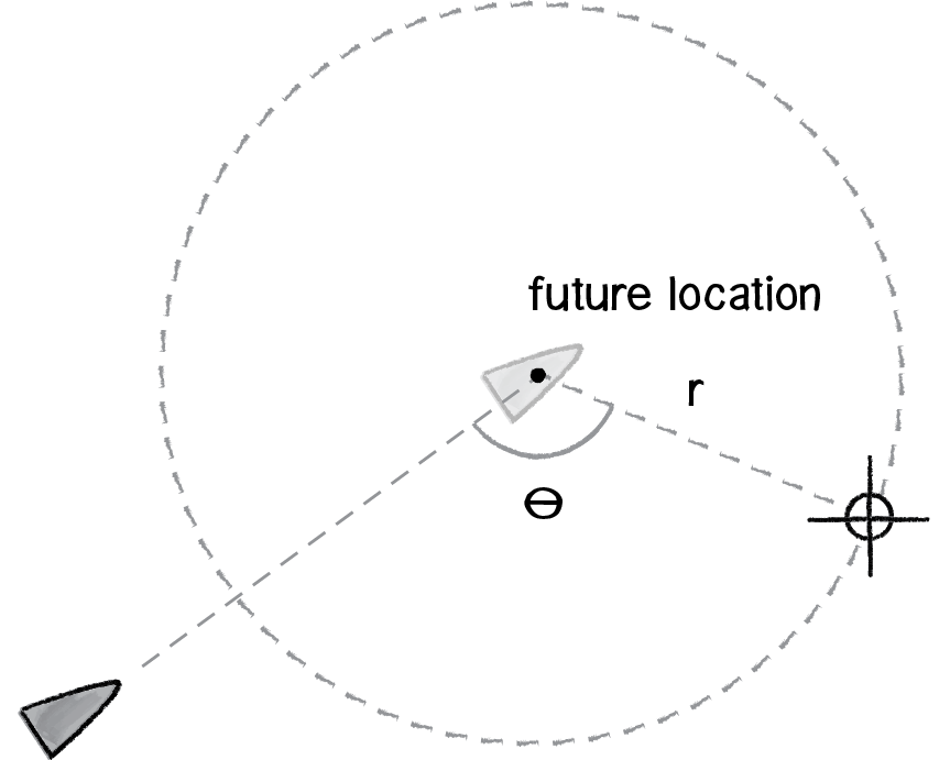
Figure 6.12

For Reynolds, the goal of wandering is not simply random motion, but rather a sense of moving in one direction for a little while, wandering off to the next for a little bit, and so on and so forth. So how does Reynolds calculate a desired vector to achieve such an effect?

Figure 6.12 illustrates how the vehicle predicts its future location as a fixed distance in front of it (in the direction of its velocity), draws a circle with radius r at that location, and picks a random point along the circumference of the circle. That random point moves randomly around the circle in each frame of animation. And that random point is the vehicle’s target, its desired vector pointing in that direction.

Sounds a bit absurd, right? Or, at the very least, rather arbitrary. In fact, this is a very clever and thoughtful solution—it uses randomness to drive a vehicle’s steering, but constrains that randomness along the path of a circle to keep the vehicle’s movement from appearing jittery, and, well, random.

But the seemingly random and arbitrary nature of this solution should drive home the point I’m trying to make—these are made-up behaviors inspired by real-life motion. You can just as easily concoct some elaborate scenario to compute a desired velocity yourself. And you should.

Let’s say we want to create a steering behavior called “stay within walls.” We’ll define the desired velocity as:

If a vehicle comes within a distance d of a wall, it desires to move at maximum speed in the opposite direction of the wall.

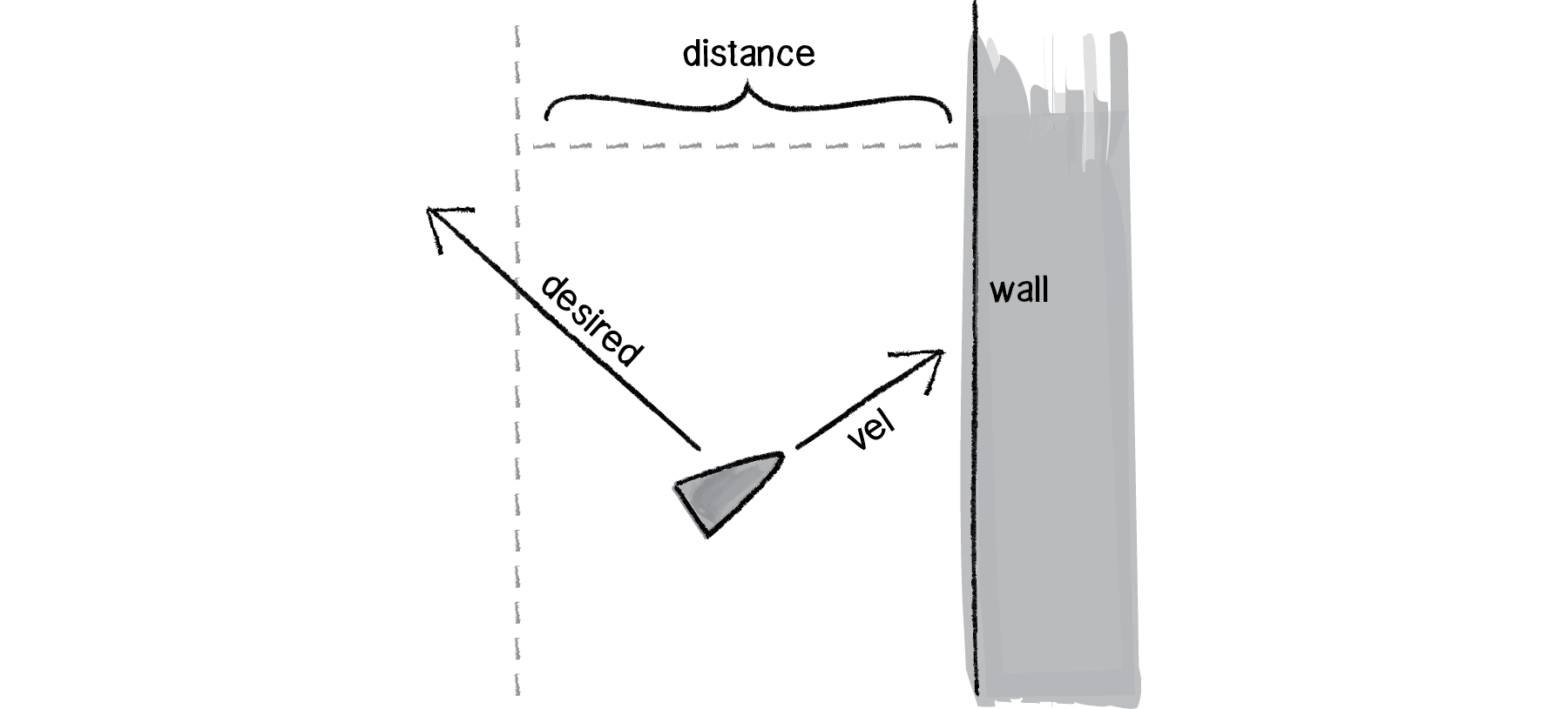
Figure 6.13

If we define the walls of the space as the edges of a Processing window and the distance d as 25, the code is rather simple.

Example 6.3: “Stay within walls” steering behavior

if (location. x > 25) {

  PVector desired = new PVector(maxspeed,velocity.y);
  PVector steer = PVector.sub(desired, velocity);
  steer.limit(maxforce);
  applyForce(steer);
}

6.6 Flow Fields

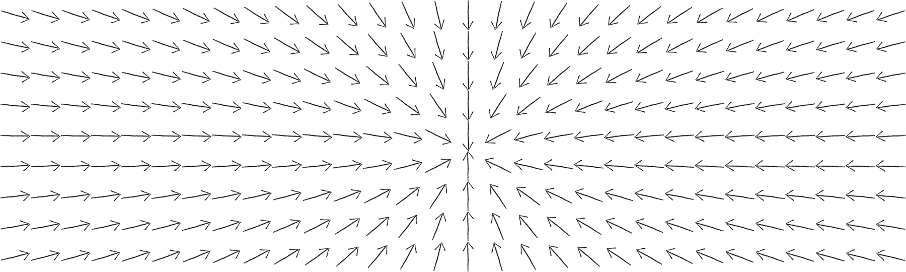
Now back to the task at hand. Let’s examine a couple more of Reynolds’s steering behaviors. First, flow field following. What is a flow field? Think of your Processing window as a grid. In each cell of the grid lives an arrow pointing in some direction—you know, a vector. As a vehicle moves around the screen, it asks, “Hey, what arrow is beneath me? That’s my desired velocity!”

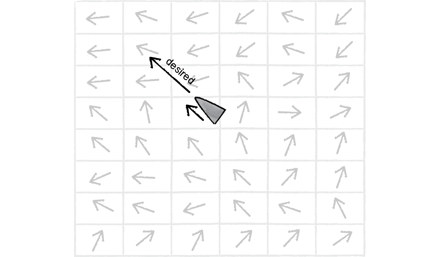
Figure 6.14

Reynolds’s flow field following example has the vehicle predicting its future location and following the vector at that spot, but for simplicity’s sake, we’ll have the vehicle simply look to the vector at its current location.

Before we can write the additional code for our Vehicle class, we’ll need to build a class that describes the flow field itself, the grid of vectors. A two-dimensional array is a convenient data structure in which to store a grid of information. If you are not familiar with 2D arrays, I suggest reviewing this online Processing tutorial: 2D array. The 2D array is convenient because we reference each element with two indices, which we can think of as columns and rows.

class FlowField {
 

  PVector[][] field;

  int cols, rows;

  int resolution;

Notice how we are defining a third variable called resolution above. What is this variable? Let’s say we have a Processing window that is 200 pixels wide by 200 pixels high. We could make a flow field that has a PVector object for every single pixel, or 40,000 PVectors (200 * 200). This isn’t terribly unreasonable, but in our case, it’s overkill. We don’t need a PVector for every single pixel; we can achieve the same effect by having, say, one every ten pixels (20 * 20 = 400). We use this resolution to define the number of columns and rows based on the size of the window divided by resolution:

  FlowField() {
    resolution = 10;

    cols = width/resolution;

    rows = height/resolution;
    field = new PVector[cols][rows];
  }

Now that we’ve set up the flow field’s data structures, it’s time to compute the vectors in the flow field itself. How do we do that? However we feel like it! Perhaps we want to have every vector in the flow field pointing to the right.

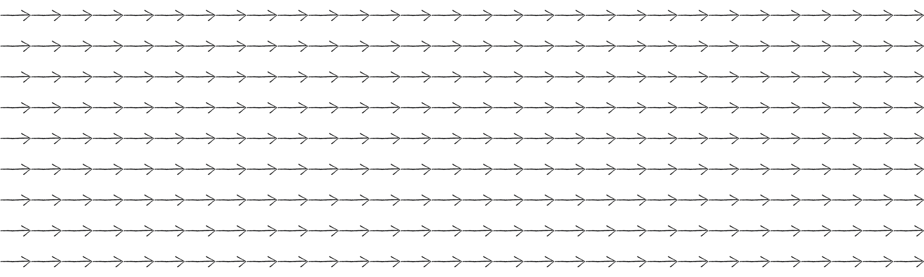
Figure 6.15

for (int i = 0; i < cols; i++) {
  for (int j = 0; j < rows; j++) {

    field[i][j] = new PVector(1,0);
  }
}

Or perhaps we want the vectors to point in random directions.

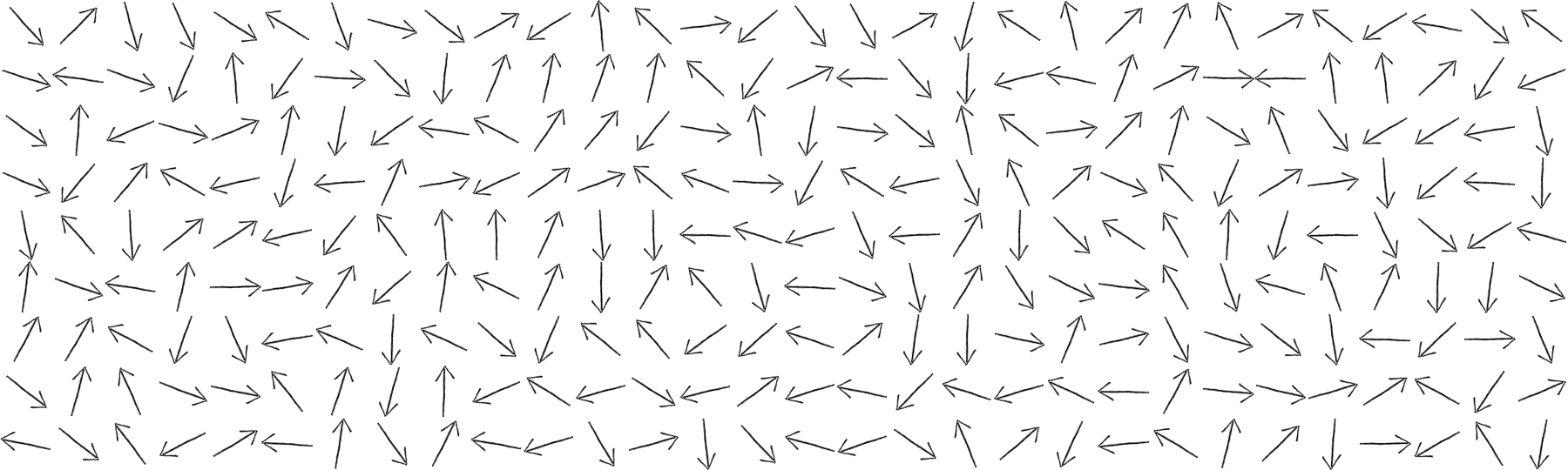
Figure 6.16

for (int i = 0; i < cols; i++) {
  for (int j = 0; j < rows; j++) {
 

    field[i][j] = PVector.2D();
  }
}

What if we use 2D Perlin noise (mapped to an angle)?

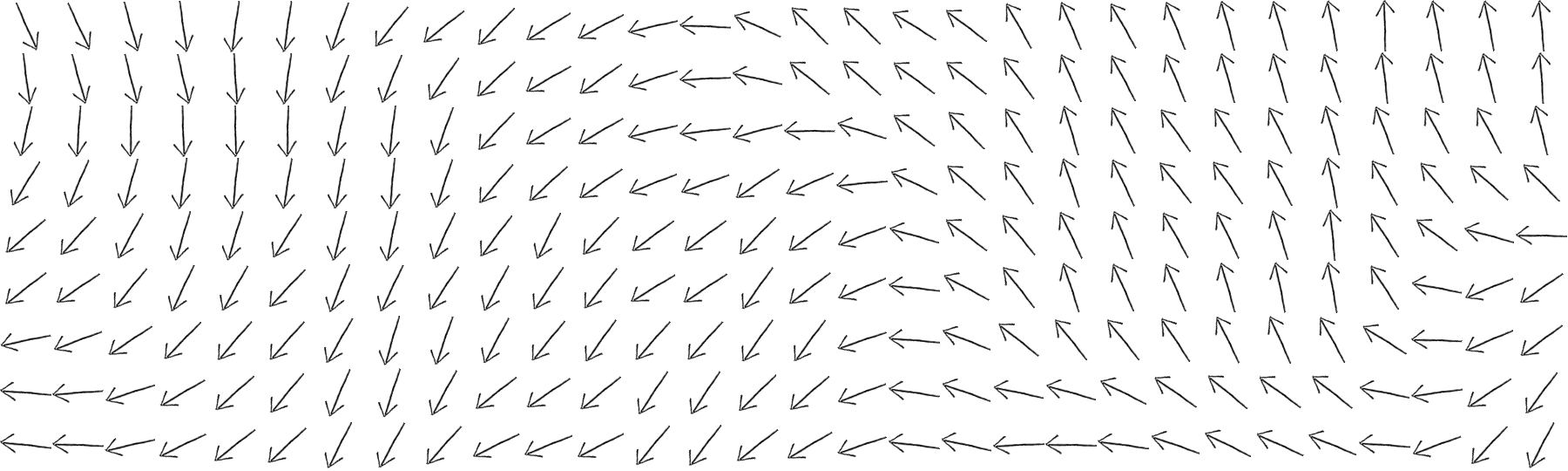
Figure 6.17

float xoff = 0;
for (int i = 0; i < cols; i++) {
  float yoff = 0;
  for (int j = 0; j < rows; j++) {

    float theta = map(noise(xoff,yoff),0,1,0,TWO_PI);
    field[i][j] = new PVector(cos(theta),sin(theta));
    yoff += 0.1;
  }
  xoff += 0.1;
}

Now we’re getting somewhere. Flow fields can be used for simulating various effects, such as an irregular gust of wind or the meandering path of a river. Calculating the direction of your vectors using Perlin noise is one way to achieve such an effect. Of course, there’s no “correct” way to calculate the vectors of a flow field; it’s really up to you to decide what you’re looking to simulate.

Exercise 6.6

Write the code to calculate a PVector at every location in the flow field that points towards the center of a window.

Show Raw PVector v = new PVector(____________,____________); v.______________(); field[i][j] = v;

PVector v = new PVector(____________,____________);
v.______________();
field[i][j] = v;

Now that we have a two-dimensional array storing all of the flow field vectors, we need a way for a vehicle to look up its desired vector in the flow field. Let’s say we have a vehicle that lives at a PVector: its location. We first need to divide by the resolution of the grid. For example, if the resolution is 10 and the vehicle is at (100,50), we need to look up column 10 and row 5.

int column = int(location.x/resolution);
int row = int(location.y/resolution);

Because a vehicle could theoretically wander off the Processing window, it’s also useful for us to employ the constrain() function to make sure we don’t look outside of the flow field array. Here is a function we’ll call lookup() that goes in the FlowField class—it receives a PVector (presumably the location of our vehicle) and returns the corresponding flow field PVector for that location.

  PVector lookup(PVector lookup) {

 
    int column = int(constrain(lookup.x/resolution,0,cols-1));
    int row = int(constrain(lookup.y/resolution,0,rows-1));

    return field[column][row].get();
  }

Before we move on to the Vehicle class, let’s take a look at the FlowField class all together.

class FlowField {
 

  PVector[][] field;
  int cols, rows;
  int resolution;
 
  FlowField(int r) {
    resolution = r;

    cols = width/resolution;
    rows = height/resolution;

    field = new PVector[cols][rows];
    init();
  }
 
  void init() {
    float xoff = 0;
    for (int i = 0; i < cols; i++) {
      float yoff = 0;
      for (int j = 0; j < rows; j++) {

        float theta = map(noise(xoff,yoff),0,1,0,TWO_PI);

        field[i][j] = new PVector(cos(theta),sin(theta));
        yoff += 0.1;
      }
      xoff += 0.1;
    }
  }
 

  PVector lookup(PVector lookup) {
 
    int column = int(constrain(lookup.x/resolution,0,cols-1));
    int row = int(constrain(lookup.y/resolution,0,rows-1));
    return field[column][row].get();
  }

}

So let’s assume we have a FlowField object called “flow”. Using the lookup() function above, our vehicle can then retrieve a desired vector from the flow field and use Reynolds’s rules (steering = desired - velocity) to calculate a steering force.

Example 6.4: Flow field following

class Vehicle {
 
  void follow(FlowField flow) {

    PVector desired = flow.lookup(location);
    desired.mult(maxspeed);
 

    PVector steer = PVector.sub(desired, velocity);
    steer.limit(maxforce);
    applyForce(steer);
  }

6.7 The Dot Product

In a moment, we’re going to work through the algorithm (along with accompanying mathematics) and code for another of Craig Reynolds’s steering behaviors: Path Following. Before we can do this, however, we have to spend some time learning about another piece of vector math that we skipped in Chapter 1—the dot product. We haven’t needed it yet, but it’s likely going to prove quite useful for you (beyond just this path-following example), so we’ll go over it in detail now.

Remember all the basic vector math we covered in Chapter 1? Add, subtract, multiply, and divide?

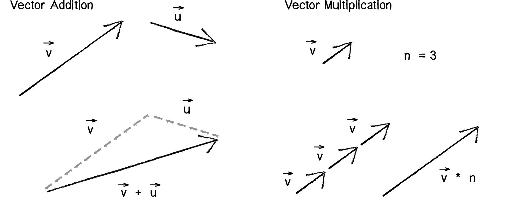
Figure 6.18

Notice how in the above diagram, vector multiplication involves multiplying a vector by a scalar value. This makes sense; when we want a vector to be twice as large (but facing the same direction), we multiply it by 2. When we want it to be half the size, we multiply it by 0.5.

However, there are two other multiplication-like operations with vectors that are useful in certain scenarios—the dot product and the cross product. For now we’re going to focus on the dot product, which is defined as follows. Assume vectors ${\displaystyle \overrightarrow{A}}$ and ${\displaystyle \overrightarrow{B}}$:

${\displaystyle \overrightarrow{A}}$ ${\displaystyle =}$ ${\displaystyle \left(a_x,a_y\right)}$
${\displaystyle \overrightarrow{B}}$ ${\displaystyle =}$ ${\displaystyle \left(b_x,b_y\right)}$

THE DOT PRODUCT: ${\displaystyle \overrightarrow{A}}$ ${\displaystyle ·}$ ${\displaystyle \overrightarrow{B}}$ ${\displaystyle =}$ ${\displaystyle a_x*b_x+a_y*b_y}$

For example, if we have the following two vectors:

${\displaystyle \overrightarrow{A}}$ ${\displaystyle =}$ ${\displaystyle \left(-3,5\right)}$
${\displaystyle \overrightarrow{B}}$ ${\displaystyle =}$ ${\displaystyle \left(10,1\right)}$

${\displaystyle \overrightarrow{A}}$ ${\displaystyle ·}$ ${\displaystyle \overrightarrow{B}}$ ${\displaystyle =}$ ${\displaystyle -3*10+5*1=-30+5=35}$

Notice that the result of the dot product is a scalar value (a single number) and not a vector.

In Processing, this would translate to:

PVector a = new PVector(-3,5);
PVector b = new PVector(10,1);
 

float n = a.dot(b);

And if we were to look in the guts of the PVector source, we’d find a pretty simple implementation of this function:

public float dot(PVector v) {
  return x*v.x + y*v.y + z*v.z;
}

This is simple enough, but why do we need the dot product, and when is it going to be useful for us in code?

One of the more common uses of the dot product is to find the angle between two vectors. Another way in which the dot product can be expressed is:

${\displaystyle \overrightarrow{A}}$ ${\displaystyle ·}$ ${\displaystyle \overrightarrow{B}}$ ${\displaystyle =}$ ${\displaystyle \parallel \overrightarrow{A}\parallel }$ ${\displaystyle *}$ ${\displaystyle \parallel \overrightarrow{B}\parallel }$ ${\displaystyle *}$ ${\displaystyle \cos \left(\theta \right)}$

In other words, A dot B is equal to the magnitude of A times magnitude of B times cosine of theta (with theta defined as the angle between the two vectors A and B).

The two formulas for dot product can be derived from one another with trigonometry, but for our purposes we can be happy with operating on the assumption that:

${\displaystyle \overrightarrow{A}}$ ${\displaystyle ·}$ ${\displaystyle \overrightarrow{B}}$ ${\displaystyle =}$ ${\displaystyle \parallel \overrightarrow{A}\parallel }$ ${\displaystyle *}$ ${\displaystyle \parallel \overrightarrow{B}\parallel }$ ${\displaystyle *}$ ${\displaystyle \cos \left(\theta \right)}$
${\displaystyle \overrightarrow{A}}$ ${\displaystyle ·}$ ${\displaystyle \overrightarrow{B}}$ ${\displaystyle =}$ ${\displaystyle a_x*b_x+a_y*b_y}$

both hold true and therefore:

${\displaystyle a_x*b_x+a_y*b_y}$ ${\displaystyle =}$ ${\displaystyle \parallel \overrightarrow{A}\parallel }$ ${\displaystyle *}$ ${\displaystyle \parallel \overrightarrow{B}\parallel }$ ${\displaystyle *}$ ${\displaystyle \cos \left(\theta \right)}$

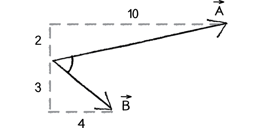
Figure 6.19

Now, let’s start with the following problem. We have the vectors A and B:

${\displaystyle \overrightarrow{A}}$ ${\displaystyle =}$ ${\displaystyle \left(10,2\right)}$
${\displaystyle \overrightarrow{B}}$ ${\displaystyle =}$ ${\displaystyle \left(4,-3\right)}$

We now have a situation in which we know everything except for theta. We know the components of the vector and can calculate the magnitude of each vector. We can therefore solve for cosine of theta:

${\displaystyle \cos \left(\theta \right)}$ ${\displaystyle =}$ ${\displaystyle (}$ ${\displaystyle \overrightarrow{A}}$ ${\displaystyle ·}$ ${\displaystyle \overrightarrow{B}}$ ${\displaystyle )}$ ${\displaystyle /}$ ${\displaystyle (}$ ${\displaystyle \parallel \overrightarrow{A}\parallel }$ ${\displaystyle *}$ ${\displaystyle \parallel \overrightarrow{B}\parallel }$ ${\displaystyle )}$

To solve for theta, we can take the inverse cosine (often expressed as cosine^-1 or arccosine).

${\displaystyle \theta }$ ${\displaystyle =}$ ${\displaystyle {\cos }^{-1}}$ ${\displaystyle (}$ ${\displaystyle (}$ ${\displaystyle \overrightarrow{A}}$ ${\displaystyle ·}$ ${\displaystyle \overrightarrow{B}}$ ${\displaystyle )}$ ${\displaystyle /}$ ${\displaystyle (}$ ${\displaystyle \parallel \overrightarrow{A}\parallel }$ ${\displaystyle *}$ ${\displaystyle \parallel \overrightarrow{B}\parallel }$ ${\displaystyle )}$ ${\displaystyle )}$

Let’s now do the math with actual numbers:

${\displaystyle \parallel \overrightarrow{A}\parallel }$ ${\displaystyle =}$ ${\displaystyle 10.2}$
${\displaystyle \parallel \overrightarrow{B}\parallel }$ ${\displaystyle =}$ ${\displaystyle 5}$

Therefore:

${\displaystyle \theta }$ ${\displaystyle =}$ ${\displaystyle {\cos }^{-1}}$ ${\displaystyle (}$ ${\displaystyle (}$ ${\displaystyle 10}$ ${\displaystyle *}$ ${\displaystyle 4}$ ${\displaystyle +}$ ${\displaystyle 2}$ ${\displaystyle *}$ ${\displaystyle -3}$ ${\displaystyle )}$ ${\displaystyle /}$ ${\displaystyle (}$ ${\displaystyle 10.2}$ ${\displaystyle *}$ ${\displaystyle 5}$ ${\displaystyle )}$ ${\displaystyle )}$
${\displaystyle \theta }$ ${\displaystyle =}$ ${\displaystyle {\cos }^{-1}}$ ${\displaystyle (}$ ${\displaystyle 34}$ ${\displaystyle /}$ ${\displaystyle 51}$ ${\displaystyle )}$
${\displaystyle \theta }$ ${\displaystyle =}$ ${\displaystyle \sim 48^{\circ }}$

The Processing version of this would be:

PVector a = new PVector(10,2);
PVector b = new PVector(4,-3);
float theta = acos(a.dot(b) / (a.mag() * b.mag()));

And, again, if we were to dig into the guts of the Processing source code, we would see a function that implements this exact algorithm.

  static public float angleBetween(PVector v1, PVector v2) {
    float dot = v1.dot(v2);
    float theta = (float) Math.acos(dot / (v1.mag() * v2.mag()));
    return theta;
  }

Exercise 6.9

Create a sketch that displays the angle between two PVector objects.

A couple things to note here:

6.8 Path Following

Now that we’ve got a basic understanding of the dot product under our belt, we can return to a discussion of Craig Reynolds’s path-following algorithm. Let’s quickly clarify something. We are talking about path following, not path finding. Pathfinding refers to a research topic (commonly studied in artificial intelligence) that involves solving for the shortest distance between two points, often in a maze. With path following, the path already exists and we’re asking a vehicle to follow that path.

Before we work out the individual pieces, let’s take a look at the overall algorithm for path following, as defined by Reynolds.

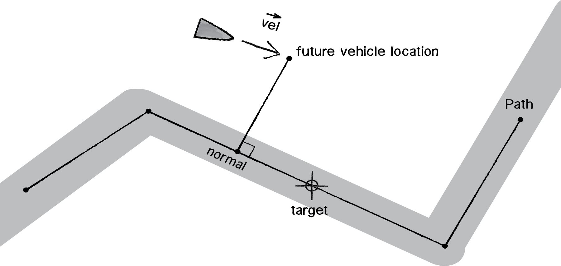
Figure 6.20

We’ll first define what we mean by a path. There are many ways we could implement a path, but for us, a simple way will be to define a path as a series of connected points:

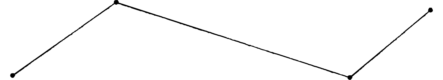
Figure 6.21: Path

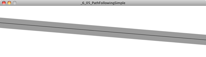
An even simpler path would be a line between two points.

Figure 6.22: Simple path

We’re also going to consider a path to have a radius. If we think of the path as a road, the radius determines the road’s width. With a smaller radius, our vehicles will have to follow the path more closely; a wider radius will allow them to stray a bit more.

Putting this into a class, we have:

class Path {
 

  PVector start;
  PVector end;

  float radius;
 
  Path() {

    radius = 20;
    start = new PVector(0,height/3);
    end = new PVector(width,2*height/3);
  }
 
  void display() {  // Display the path.
    strokeWeight(radius*2);
    stroke(0,100);
    line(start.x,start.y,end.x,end.y);
    strokeWeight(1);
    stroke(0);
    line(start.x,start.y,end.x,end.y);
  }
}

Now, let’s assume we have a vehicle (as depicted below) outside of the path’s radius, moving with a velocity.

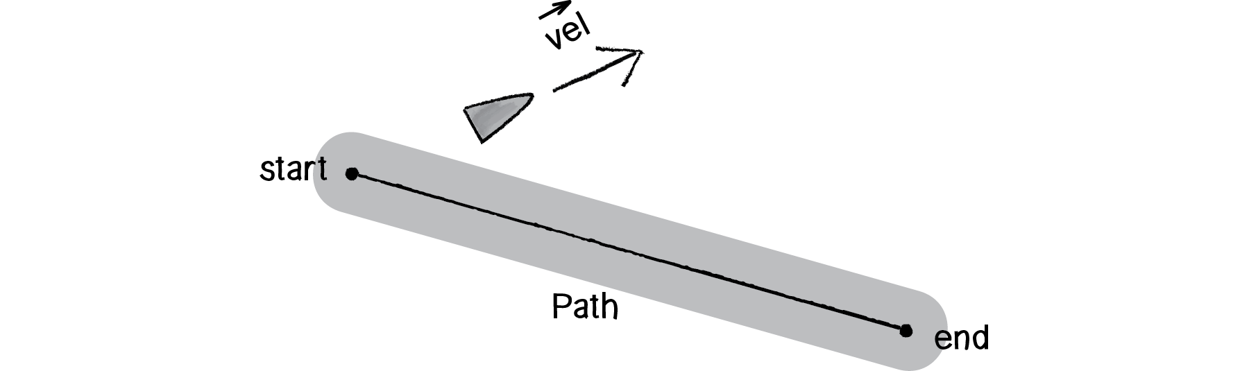
Figure 6.23

The first thing we want to do is predict, assuming a constant velocity, where that vehicle will be in the future.

PVector predict = vel.get();
 

predict.normalize();
predict.mult(25);

PVector predictLoc = PVector.add(loc, predict);

Once we have that location, it’s now our job to find out the vehicle’s current distance from the path of that predicted location. If it’s very far away, well, then, we’ve strayed from the path and need to steer back towards it. If it’s close, then we’re doing OK and are following the path nicely.

So, how do we find the distance between a point and a line? This concept is key. The distance between a point and a line is defined as the length of the normal between that point and line. The normal is a vector that extends from that point and is perpendicular to the line.

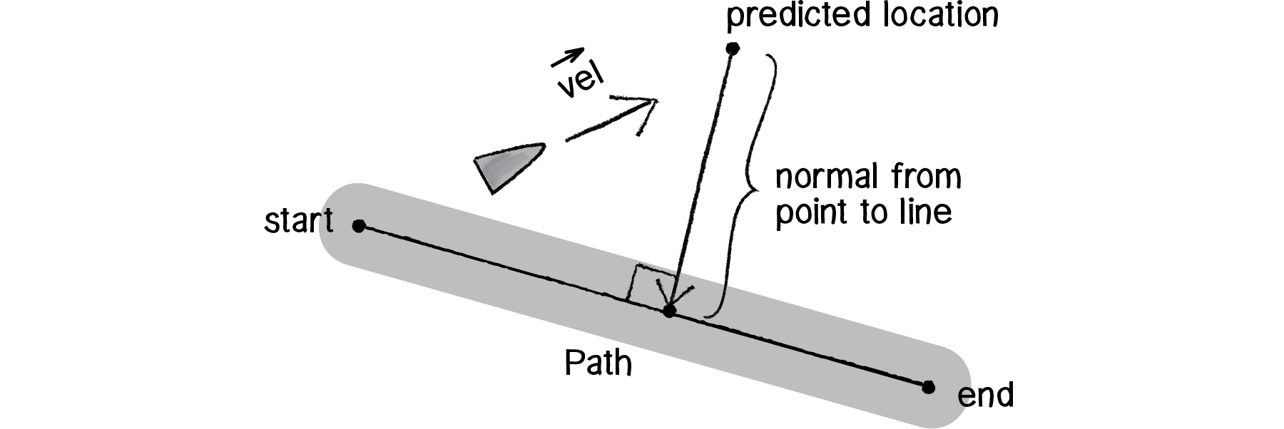
Figure 6.24

Let’s figure out what we do know. We know we have a vector (call it ${\displaystyle \overrightarrow{A}}$) that extends from the path’s starting point to the vehicle’s predicted location.

PVector a = PVector.sub(predictLoc,path.start);

We also know that we can define a vector (call it ${\displaystyle \overrightarrow{B}}$) that points from the start of the path to the end.

PVector b = PVector.sub(path.end,path.start);

Now, with basic trigonometry, we know that the distance from the path’s start to the normal point is: |A| * cos(theta).

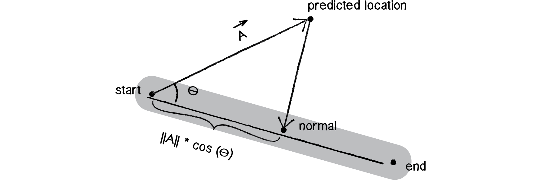
Figure 6.25

If we knew theta, we could easily define that normal point as follows:

float d = a.mag()*cos(theta);
b.normalize();

b.mult(d);

PVector normalPoint = PVector.add(path.start,b);

And if the dot product has taught us anything, it’s that given two vectors, we can get theta, the angle between.

float theta = PVector.angleBetween(a,b);
b.normalize();
b.mult(a.mag()*cos(theta));
PVector normalPoint = PVector.add(path.start,b);

While the above code will work, there’s one more simplification we can make. If you’ll notice, the desired magnitude for vector ${\displaystyle \overrightarrow{B}}$ is:

a.mag()*cos(theta)

which is the code translation of:

${\displaystyle \parallel \overrightarrow{A}\parallel }$ ${\displaystyle *}$ ${\displaystyle \cos \left(\theta \right)}$

And if you recall:

${\displaystyle \overrightarrow{A}}$ ${\displaystyle ·}$ ${\displaystyle \overrightarrow{B}}$ ${\displaystyle =}$ ${\displaystyle \parallel \overrightarrow{A}\parallel }$ ${\displaystyle *}$ ${\displaystyle \parallel \overrightarrow{B}\parallel }$ ${\displaystyle *}$ ${\displaystyle \cos \left(\theta \right)}$

Now, what if vector ${\displaystyle \overrightarrow{B}}$ is a unit vector, i.e. length 1? Then:

${\displaystyle \overrightarrow{A}}$ ${\displaystyle ·}$ ${\displaystyle \overrightarrow{B}}$ ${\displaystyle =}$ ${\displaystyle \parallel \overrightarrow{A}\parallel }$ ${\displaystyle *}$ ${\displaystyle 1}$ ${\displaystyle *}$ ${\displaystyle \cos \left(\theta \right)}$

or

${\displaystyle \overrightarrow{A}}$ ${\displaystyle ·}$ ${\displaystyle \overrightarrow{B}}$ ${\displaystyle =}$ ${\displaystyle \parallel \overrightarrow{A}\parallel }$ ${\displaystyle *}$ ${\displaystyle \cos \left(\theta \right)}$

And what are we doing in our code? Normalizing b!

b.normalize();

Because of this fact, we can simplify our code as:

float theta = PVector.angleBetween(a,b);
 
b.normalize();

b.mult(a.dot(b));
 
PVector normalPoint = PVector.add(path.start,b);

This process is commonly known as “scalar projection.” |A| cos(θ) is the scalar projection of A onto B.

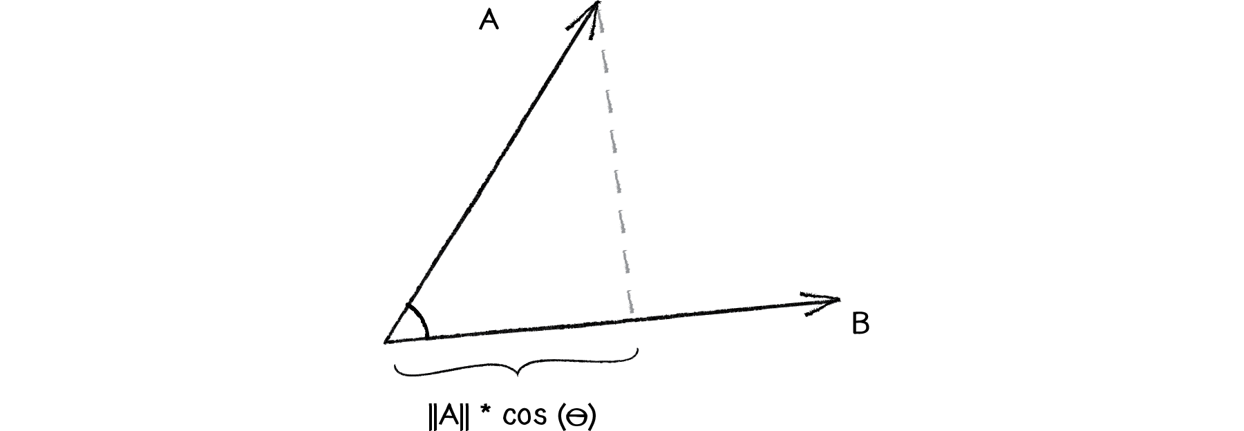
Figure 6.26

Once we have the normal point along the path, we have to decide whether the vehicle should steer towards the path and how. Reynolds’s algorithm states that the vehicle should only steer towards the path if it strays beyond the path (i.e., if the distance between the normal point and the predicted future location is greater than the path radius).

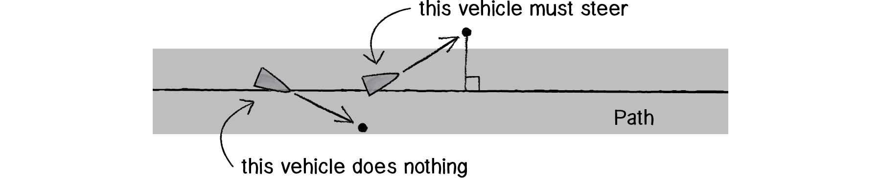
Figure 6.27

float distance = PVector.dist(predictLoc, normalPoint);
 

if (distance > path.radius) {

  seek(target);
}

But what is the target?

Reynolds’s algorithm involves picking a point ahead of the normal on the path (see step #3 above). But for simplicity, we could just say that the target is the normal itself. This will work fairly well:

float distance = PVector.dist(predictLoc, normalPoint);
if (distance > path.radius) {

  seek(normalPoint);
}

Since we know the vector that defines the path (we’re calling it “B”), we can implement Reynolds’s “point ahead on the path” without too much trouble.

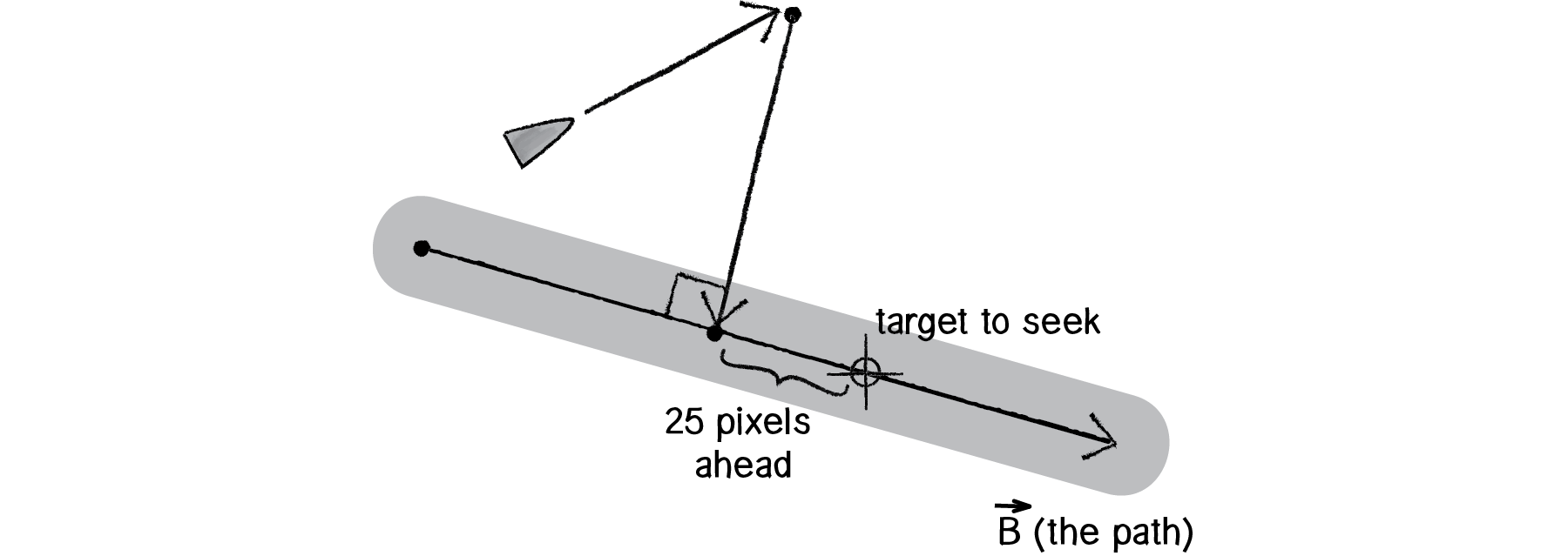
Figure 6.28

float distance = PVector.dist(predictLoc, normalPoint);
if (distance > path.radius) {

  b.normalize();
  b.mult(25);

  PVector target = PVector.add(normalPoint,b);
 
  seek(target);
}

Putting it all together, we have the following steering function in our Vehicle class.

Example 6.5: Simple path following

  void follow(Path p) {
 

    PVector predict = vel.get();
    predict.normalize();
    predict.mult(25);
    PVector predictLoc = PVector.add(loc, predict);

    PVector a = p.start;
    PVector b = p.end;
    PVector normalPoint = getNormalPoint(predictLoc, a, b);

    PVector dir = PVector.sub(b, a);
    dir.normalize();
    dir.mult(10);
    PVector target = PVector.add(normalPoint, dir);

    float distance =
      PVector.dist(normalPoint, predictLoc);
    if (distance > p.radius) {
      seek(target);
    }
  }

Now, you may notice above that instead of using all that dot product/scalar projection code to find the normal point, we instead call a function: getNormalPoint(). In cases like this, it’s useful to break out the code that performs a specific task (finding a normal point) into a function that it can be used generically in any case where it is required. The function takes three PVectors: the first defines a point in Cartesian space and the second and third arguments define a line segment.

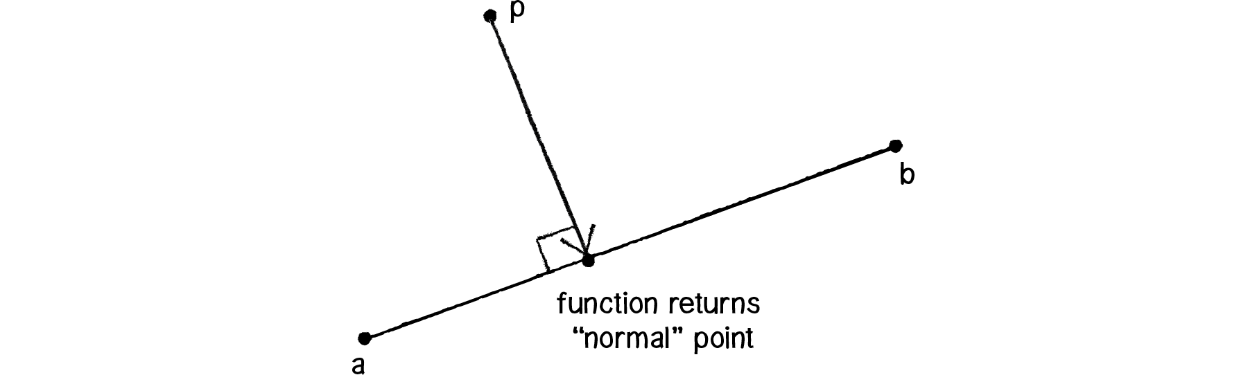
Figure 6.29

  PVector getNormalPoint(PVector p, PVector a, PVector b) {

    PVector ap = PVector.sub(p, a);

    PVector ab = PVector.sub(b, a);
 

    ab.normalize();
    ab.mult(ap.dot(ab));

    PVector normalPoint = PVector.add(a, ab);
 
    return normalPoint;
  }

What do we have so far? We have a Path class that defines a path as a line between two points. We have a Vehicle class that defines a vehicle that can follow the path (using a steering behavior to seek a target along the path). What is missing?

Take a deep breath. We’re almost there.

6.9 Path Following with Multiple Segments

Figure 6.30

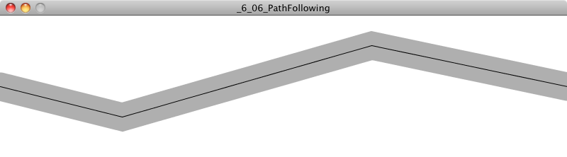
We’ve built a great example so far, yes, but it’s pretty darn limiting. After all, what if we want our path to be something that looks more like:

Figure 6.31

While it’s true that we could make this example work for a curved path, we’re much less likely to end up needing a cool compress on our forehead if we stick with line segments. In the end, we can always employ the same technique we discovered with Box2D—we can draw whatever fancy curved path we want and approximate it behind the scenes with simple geometric forms.

So, what’s the problem? If we made path following work with one line segment, how do we make it work with a series of connected line segments? Let’s take a look again at our vehicle driving along the screen. Say we arrive at Step 3.

Step 3: Find a target point on the path.

To find the target, we need to find the normal to the line segment. But now that we have a series of line segments, we have a series of normal points (see above)! Which one do we choose? The solution we’ll employ is to pick the normal point that is (a) closest and (b) on the path itself.

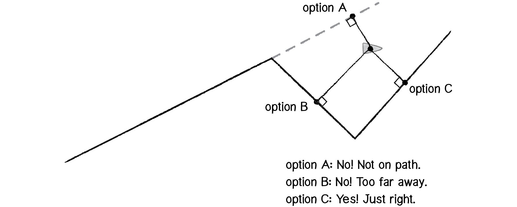
Figure 6.32

If we have a point and an infinitely long line, we’ll always have a normal. But, as in the path-following example, if we have a point and a line segment, we won’t necessarily find a normal that is on the line segment itself. So if this happens for any of the segments, we can disqualify those normals. Once we are left with normals that are on the path itself (only two in the above diagram), we simply pick the one that is closest to our vehicle’s location.

In order to write the code for this, we’ll have to expand our Path class to have an ArrayList of points (rather than just two, a start and an end).

 class Path {
 

  ArrayList<PVector> points;
  float radius;
 
  Path() {
    radius = 20;
    points = new ArrayList<PVector>();
  }
 

  void addPoint(float x, float y) {   .
    PVector point = new PVector(x,y);
    points.add(point);
  }

  void display() {
    stroke(0);
    noFill();
    beginShape();
    for (PVector v : points) {
      vertex(v.x,v.y);
    }
    endShape();
  }

}

Now that we have the Path class defined, it’s the vehicle’s turn to deal with multiple line segments. All we did before was find the normal for one line segment. We can now find the normals for all the line segments in a loop.

for (int i = 0; i < p.points.size()-1; i++) {
  PVector a = p.points.get(i);
  PVector b = p.points.get(i+1);

  PVector normalPoint = getNormalPoint(predictLoc, a, b);

Then we should make sure the normal point is actually between points a and b. Since we know our path goes from left to right in this example, we can test if the x component of normalPoint is outside the x components of a and b.

   if (normalPoint.x < a.x || normalPoint.x > b.x) {

      normalPoint = b.get();
   }

As a little trick, we’ll say that if it’s not within the line segment, let’s just pretend the end point of that line segment is the normal. This will ensure that our vehicle always stays on the path, even if it strays out of the bounds of our line segments.

Finally, we’ll need to make sure we find the normal point that is closest to our vehicle. To accomplish this, we start with a very high “world record” distance and iterate through each normal point to see if it beats the record (i.e. is less than). Each time a normal point beats the record, the world record is updated and the winning point is stored in a variable named target. At the end of the loop, we’ll have the closest normal point in that variable.

Example 6.6: Path following

PVector target = null;

float worldRecord = 1000000;
 
for (int i = 0; i < p.points.size()-1; i++) {
  PVector a = p.points.get(i);
  PVector b = p.points.get(i+1);
  PVector normalPoint = getNormalPoint(predictLoc, a, b);
  if (normalPoint.x < a.x || normalPoint.x > b.x) {
    normalPoint = b.get();
  }
 
  float distance = PVector.dist(predictLoc, normalPoint);
 

  if (distance < worldRecord) {
    worldRecord = distance;
    target = normalPoint.get();
  }

}

if (normalPoint.x < ____(____,____) || normalPoint.x > ____(____,____)) {
  normalPoint = b.get();
}

6.10 Complex Systems

Remember our purpose? To breathe life into the things that move around our Processing windows? By learning to write the code for an autonomous agent and building a series of examples of individual behaviors, hopefully our souls feel a little more full. But this is no place to stop and rest on our laurels. We’re just getting started. After all, there is a deeper purpose at work here. Yes, a vehicle is a simulated being that makes decisions about how to seek and flow and follow. But what is a life led alone, without the love and support of others? Our purpose here is not only to build individual behaviors for our vehicles, but to put our vehicles into systems of many vehicles and allow those vehicles to interact with each other.

Let’s think about a tiny, crawling ant—one single ant. An ant is an autonomous agent; it can perceive its environment (using antennae to gather information about the direction and strength of chemical signals) and make decisions about how to move based on those signals. But can a single ant acting alone build a nest, gather food, defend its queen? An ant is a simple unit and can only perceive its immediate environment. A colony of ants, however, is a sophisticated complex system, a “superorganism” in which the components work together to accomplish difficult and complicated goals.

We want to take what we’ve learned during the process of building autonomous agents in Processing into simulations that involve many agents operating in parallel—agents that have an ability to perceive not only their physical environment but also the actions of their fellow agents, and then act accordingly. We want to create complex systems in Processing.

What is a complex system? A complex system is typically defined as a system that is “more than the sum of its parts.” While the individual elements of the system may be incredibly simple and easily understood, the behavior of the system as a whole can be highly complex, intelligent, and difficult to predict. Here are three key principles of complex systems.

Following are three additional features of complex systems that will help frame the discussion, as well as provide guidelines for features we will want to include in our software simulations. It’s important to acknowledge that this is a fuzzy set of characteristics and not all complex systems have all of them.

Complexity will serve as a theme for the remaining content in this book. In this chapter, we’ll begin by adding one more feature to our Vehicle class: an ability to look at neighboring vehicles.

6.11 Group Behaviors (or: Let’s not run into each other)

A group is certainly not a new concept. We’ve done this before—in Chapter 4, where we developed a framework for managing collections of particles in a ParticleSystem class. There, we stored a list of particles in an ArrayList. We’ll do the same thing here: store a bunch of Vehicle objects in an ArrayList.

ArrayList<Vehicle> vehicles;
 
void setup() {

  vehicles = new ArrayList<Vehicle>;
  for (int i = 0; i < 100; i++) {
    vehicles.add(new Vehicle(random(width),random(height)));
  }
}

Now when it comes time to deal with all the vehicles in draw(), we simply loop through all of them and call the necessary functions.

void draw(){
  for (Vehicle v : vehicles) {
    v.update();
    v.display();
  }
}

OK, so maybe we want to add a behavior, a force to be applied to all the vehicles. This could be seeking the mouse.

    v.seek(mouseX,mouseY);

But that’s an individual behavior. We’ve already spent thirty-odd pages worrying about individual behaviors. We’re here because we want to apply a group behavior. Let’s begin with separation, a behavior that commands, “Avoid colliding with your neighbors!”

    v.separate();

Is that right? It sounds good, but it’s not. What’s missing? In the case of seek, we said, “Seek mouseX and mouseY.” In the case of separate, we’re saying “separate from everyone else.” Who is everyone else? It’s the list of all the other vehicles.

    v.separate(vehicles);

This is the big leap beyond what we did before with particle systems. Instead of having each element (particle or vehicle) operate on its own, we’re now saying, “Hey you, the vehicle! When it comes time for you to operate, you need to operate with an awareness of everyone else. So I’m going to go ahead and pass you the ArrayList of everyone else.”

This is how we’ve mapped out setup() and draw() to deal with a group behavior.

ArrayList<Vehicle> vehicles;
 
void setup() {
  size(320,240);
  vehicles = new ArrayList<Vehicle>();
  for (int i = 0; i < 100; i++) {
    vehicles.add(new Vehicle(random(width),random(height)));
  }
}
 
void draw() {
  background(255);
 
  for (Vehicle v : vehicles) {

    v.separate(vehicles);
    v.update();
    v.display();
  }
}

Figure 6.33

Of course, this is just the beginning. The real work happens inside the separate() function itself. Let’s figure out how we want to define separation. Reynolds states: “Steer to avoid crowding.” In other words, if a given vehicle is too close to you, steer away from that vehicle. Sound familiar? Remember the seek behavior where a vehicle steers towards a target? Reverse that force and we have the flee behavior.

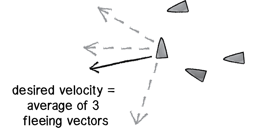
Figure 6.34

But what if more than one vehicle is too close? In this case, we’ll define separation as the average of all the vectors pointing away from any close vehicles.

Let’s begin to write the code. As we just worked out, we’re writing a function called separate() that receives an ArrayList of Vehicle objects as an argument.

void separate (ArrayList<Vehicle> vehicles) {
 
}

Inside this function, we’re going to loop through all of the vehicles and see if any are too close.

  float desiredseparation = 20;
 
  for (Vehicle other : vehicles) {
 

    float d = PVector.dist(location, other.location);
 
 
    if ((d > 0) && (d < desiredseparation)) {

 
    }
  }

Notice how in the above code, we are not only checking if the distance is less than a desired separation (i.e. too close!), but also if the distance is greater than zero. This is a little trick that makes sure we don’t ask a vehicle to separate from itself. Remember, all the vehicles are in the ArrayList, so if you aren’t careful you’ll be comparing each vehicle to itself!

Once we know that two vehicles are too close, we need to make a vector that points away from the offending vehicle.

    if ((d > 0) && (d < desiredseparation)) {

      PVector diff = PVector.sub(location, other.location);
      diff.normalize();
    }

This is not enough. We have that vector now, but we need to make sure we calculate the average of all vectors pointing away from close vehicles. How do we compute average? We add up all the vectors and divide by the total.

  PVector sum = new PVector();
  int count = 0;

  for (Vehicle other : vehicles) {
 
    float d = PVector.dist(location, other.location);
    if ((d > 0) && (d < desiredseparation)) {
      PVector diff = PVector.sub(location, other.location);
      diff.normalize();

      sum.add(diff);
      count++;
    }
  }
 

  if (count > 0) {
    sum.div(count);
  }

Once we have the average vector (stored in the PVector object “sum”), that PVector can be scaled to maximum speed and become our desired velocity—we desire to move in that direction at maximum speed! And once we have the desired velocity, it’s the same old Reynolds story: steering equals desired minus velocity.

  if (count > 0) {
    sum.div(count);
 

    sum.setMag(maxspeed);
 

    PVector steer = PVector.sub(sum,vel);
    steer.limit(maxforce);
 

    applyForce(steer);
  }

Let’s see the function in its entirety. There are two additional improvements, noted in the code comments.

Example 6.7: Group behavior: Separation

  void separate (ArrayList<Vehicle> vehicles) {

    float desiredseparation = r*2;
    PVector sum = new PVector();
    int count = 0;
    for (Vehicle other : vehicles) {
      float d = PVector.dist(location, other.location);
      if ((d > 0) && (d < desiredseparation)) {
        PVector diff = PVector.sub(location, other.location);
        diff.normalize();

        diff.div(d);
        sum.add(diff);
        count++;
 
      }
    }
    if (count > 0) {
      sum.div(count);
      sum.normalize();
      sum.mult(maxspeed);
      PVector steer = PVector.sub(sum, vel);
      steer.limit(maxforce);
      applyForce(steer);
    }
 
  }

6.12 Combinations

The previous two exercises hint at what is perhaps the most important aspect of this chapter. After all, what is a Processing sketch with one steering force compared to one with many? How could we even begin to simulate emergence in our sketches with only one rule? The most exciting and intriguing behaviors will come from mixing and matching multiple steering forces, and we’ll need a mechanism for doing so.

You may be thinking, “Duh, this is nothing new. We do this all the time.” You would be right. In fact, we did this as early as Chapter 2.

  PVector wind = new PVector(0.001,0);
  PVector gravity = new PVector(0,0.1);
  mover.applyForce(wind);
  mover.applyForce(gravity);

Here we have a mover that responds to two forces. This all works nicely because of the way we designed the Mover class to accumulate the force vectors into its acceleration vector. In this chapter, however, our forces stem from internal desires of the movers (now called vehicles). And those desires can be weighted. Let’s consider a sketch where all vehicles have two desires:

We might begin by adding a function to the Vehicle class that manages all of the behaviors. Let’s call it applyBehaviors().

void applyBehaviors(ArrayList<Vehicle> vehicles) {
  separate(vehicles);
  seek(new PVector(mouseX,mouseY));
}

Here we see how a single function takes care of calling the other functions that apply the forces—separate() and seek(). We could start mucking around with those functions and see if we can adjust the strength of the forces they are calculating. But it would be easier for us to ask those functions to return the forces so that we can adjust their strength before applying them to the vehicle’s acceleration.

  void applyBehaviors(ArrayList<Vehicle> vehicles) {
    PVector separate = separate(vehicles);
    PVector seek = seek(new PVector(mouseX,mouseY));

    applyForce(separate);
    applyForce(seek);

  }

Let’s look at how the seek function changed.

  PVector seek(PVector target) {
    PVector desired = PVector.sub(target,loc);
    desired.normalize();
    desired.mult(maxspeed);
    PVector steer = PVector.sub(desired,vel);
    steer.limit(maxforce);
 

    applyForce(steer);
    return steer;

  }

This is a subtle change, but incredibly important for us: it allows us to alter the strength of these forces in one place.

Example 6.8: Combining steering behaviors: Seek and separate

void applyBehaviors(ArrayList<Vehicle> vehicles) {
  PVector separate = separate(vehicles);
  PVector seek = seek(new PVector(mouseX,mouseY));
 

  separate.mult(1.5);
  seek.mult(0.5);
 
 

  applyForce(separate);
  applyForce(seek);
}

6.13 Flocking

Flocking is an group animal behavior that is characteristic of many living creatures, such as birds, fish, and insects. In 1986, Craig Reynolds created a computer simulation of flocking behavior and documented the algorithm in his paper, “Flocks, Herds, and Schools: A Distributed Behavioral Model.” Recreating this simulation in Processing will bring together all the concepts in this chapter.

The good news is, we’ve already done items 1 through 3 in this chapter, so this section will be about just putting it all together and seeing the result.

Before we begin, I should mention that we’re going to change the name of our Vehicle class (yet again). Reynolds uses the term “boid” (a made-up word that refers to a bird-like object) to describe the elements of a flocking system and we will do the same.

Let’s take an overview of the three rules of flocking.

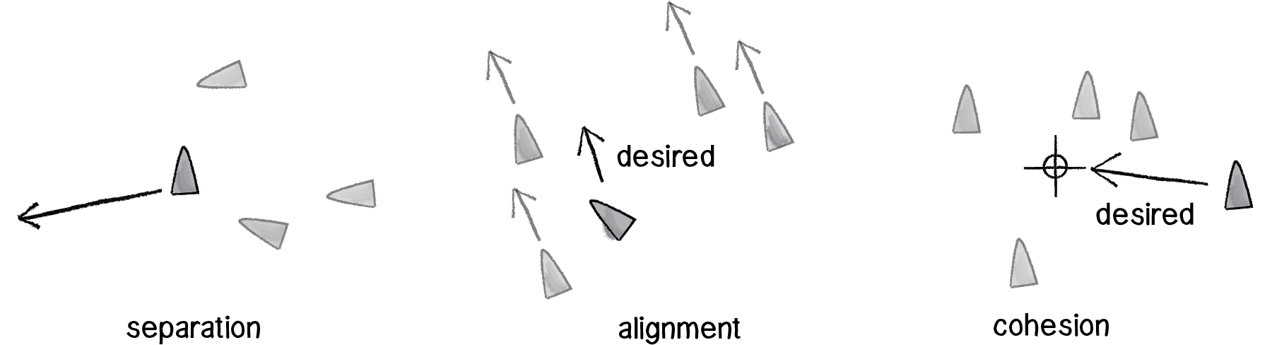
Figure 6.35

Just as we did with our separate and seek example, we’ll want our Boid objects to have a single function that manages all the above behaviors. We’ll call this function flock().

  void flock(ArrayList<Boid> boids) {

    PVector sep = separate(boids);
    PVector ali = align(boids);
    PVector coh = cohesion(boids);

    sep.mult(1.5);
    ali.mult(1.0);
    coh.mult(1.0);

    applyForce(sep);
    applyForce(ali);
    applyForce(coh);

  }

Now, it’s just a matter of implementing the three rules. We did separation before; it’s identical to our previous example. Let’s take a look at alignment, or steering in the same direction as your neighbors. As with all of our steering behaviors, we’ve got to boil down this concept into a desire: the boid’s desired velocity is the average velocity of its neighbors.

So our algorithm is to calculate the average velocity of all the other boids and set that to desired.

  PVector align (ArrayList<Boid> boids) {

    PVector sum = new PVector(0,0);
    for (Boid other : boids) {
      sum.add(other.velocity);
    }
    sum.div(boids.size());

    sum.setMag(maxspeed);
 

    PVector steer = PVector.sub(sum,velocity);
    steer.limit(maxforce);
    return steer;
  }

The above is pretty good, but it’s missing one rather crucial detail. One of the key principles behind complex systems like flocking is that the elements (in this case, boids) have short-range relationships. Thinking about ants again, it’s pretty easy to imagine an ant being able to sense its immediate environment, but less so an ant having an awareness of what another ant is doing hundreds of feet away. The fact that the ants can perform such complex collective behavior from only these neighboring relationships is what makes them so exciting in the first place.

In our alignment function, we’re taking the average velocity of all the boids, whereas we should really only be looking at the boids within a certain distance. That distance threshold is up to you, of course. You could design boids that can see only twenty pixels away or boids that can see a hundred pixels away.

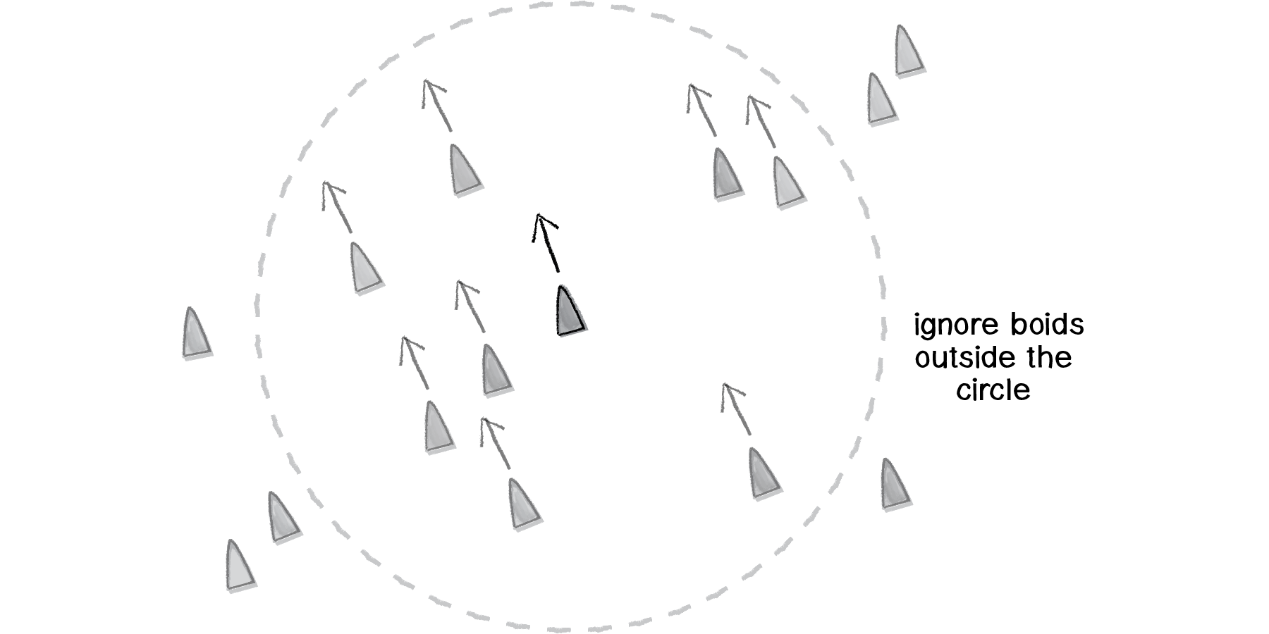
Figure 6.36

Much like we did with separation (only calculating a force for others within a certain distance), we’ll want to do the same with alignment (and cohesion).

  PVector align (ArrayList<Boid> boids) {

    float neighbordist = 50;
    PVector sum = new PVector(0,0);
    int count = 0;
    for (Boid other : boids) {
      float d = PVector.dist(location,other.location);
      if ((d > 0) && (d < neighbordist)) {
        sum.add(other.velocity);

        count++;
      }
    }
    if (count > 0) {
      sum.div(count);
      sum.normalize();
      sum.mult(maxspeed);
      PVector steer = PVector.sub(sum,velocity);
      steer.limit(maxforce);
      return steer;

    } else {
      return new PVector(0,0);
    }

  }

Exercise 6.15

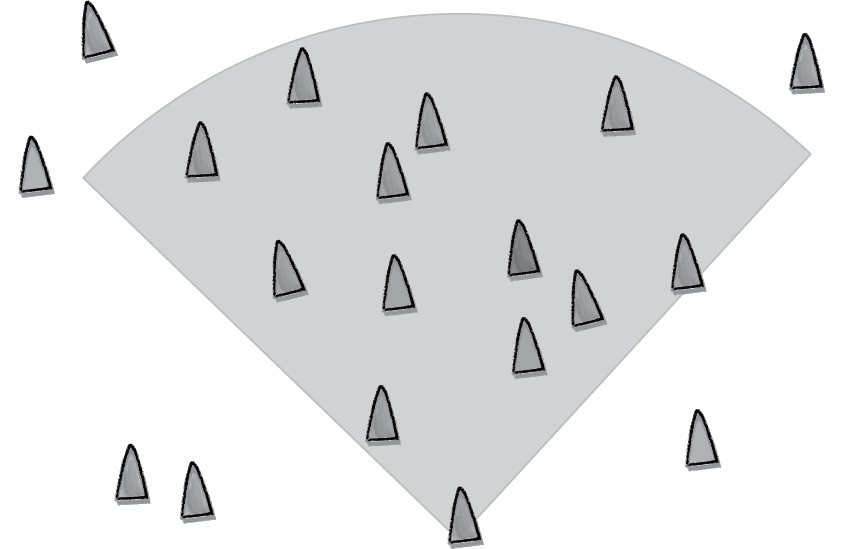
Can you write the above code so that boids can only see other boids that are actually within their “peripheral” vision (as if they had eyes)?

Finally, we are ready for cohesion. Here our code is virtually identical to that for alignment—only instead of calculating the average velocity of the boid’s neighbors, we want to calculate the average location of the boid’s neighbors (and use that as a target to seek).

  PVector cohesion (ArrayList<Boid> boids) {
    float neighbordist = 50;
    PVector sum = new PVector(0,0);
    int count = 0;
    for (Boid other : boids) {
      float d = PVector.dist(location,other.location);
      if ((d > 0) && (d < neighbordist)) {

        sum.add(other.location);
        count++;
      }
    }
    if (count > 0) {
      sum.div(count);

      return seek(sum);
    } else {
      return new PVector(0,0);
    }
  }

It’s also worth taking the time to write a class called Flock, which will be virtually identical to the ParticleSystem class we wrote in Chapter 4 with only one tiny change: When we call run() on each Boid object (as we did to each Particle object), we’ll pass in a reference to the entire ArrayList of boids.

class Flock {
  ArrayList<Boid> boids;
 
  Flock() {
    boids = new ArrayList<Boid>();
  }
 
  void run() {
    for (Boid b : boids) {

      b.run(boids);
    }
  }
 
  void addBoid(Boid b) {
    boids.add(b);
  }
}

And our main program will look like:

Example 6.9: Flocking

Flock flock;
void setup() {
  size(300,200);
  flock = new Flock();
  for (int i = 0; i < 100; i++) {
    Boid b = new Boid(width/2,height/2);

    flock.addBoid(b);
  }
}
 
void draw() {
  background(255);
  flock.run();
}

Exercise 6.17

In his book The Computational Beauty of Nature (MIT Press, 2000), Gary Flake describes a fourth rule for flocking: “View: move laterally away from any boid that blocks the view.” Have your boids follow this rule.

6.14 Algorithmic Efficiency (or: Why does my $@(*%! run so slowly?)

I would like to hide the dark truth behind we’ve just done, because I would like you to be happy and live a fulfilling and meaningful life. But I also would like to be able to sleep at night without worrying about you so much. So it is with a heavy heart that I must bring up this topic. Group behaviors are wonderful. But they can be slow, and the more elements in the group, the slower they can be. Usually, when we talk about Processing sketches running slowly, it’s because drawing to the screen can be slow—the more you draw, the slower your sketch runs. This is actually a case, however, where the slowness derives from the algorithm itself. Let’s discuss.

Computer scientists classify algorithms with something called “Big O notation,” which describes the efficiency of an algorithm: how many computational cycles does it require to complete? Let’s consider a simple analog search problem. You have a basket containing one hundred chocolate treats, only one of which is pure dark chocolate. That’s the one you want to eat. To find it, you pick the chocolates out of the basket one by one. Sure, you might be lucky and find it on the first try, but in the worst-case scenario you have to check all one hundred before you find the dark chocolate. To find one thing in one hundred, you have to check one hundred things (or to find one thing in N things, you have to check N times.) Your Big O Notation is N. This, incidentally, is the Big O Notation that describes our simple particle system. If we have N particles, we have to run and display those particles N times.

Now, let’s think about a group behavior (such as flocking). For every Boid object, we have to check every other Boid object (for its velocity and location). Let’s say we have one hundred boids. For boid #1, we need to check one hundred boids; for boid #2, we need to check one hundred boids, and so on and so forth. For one hundred boids, we need to perform one hundred times one hundred checks, or ten thousand. No problem: computers are fast and can do things ten thousand times pretty easily. Let’s try one thousand.

1,000 x 1,000 = 1,000,000 cycles.

OK, this is rather slow, but still somewhat manageable. Let’s try 10,000 elements:

10,000 x 10,000 elements = 100,000,000 cycles.

Now, we’re really getting slow. Really, really, really slow.

Notice something odd? As the number of elements increases by a factor of 10, the number of required cycles increases by a factor of 100. Or as the number of elements increases by a factor of N, the cycles increase by a factor of N times N. This is known as Big O Notation N-Squared.

I know what you are thinking. You are thinking: “No problem; with flocking, we only need to consider the boids that are close to other boids. So even if we have 1,000 boids, we can just look at, say, the 5 closest boids and then we only have 5,000 cycles.” You pause for a moment, and then start thinking: “So for each boid I just need to check all the boids and find the five closest ones and I’m good!” See the catch-22? Even if we only want to look at the close ones, the only way to know what the close ones are would be to check all of them.

Or is there another way?

Let’s take a number that we might actually want to use, but would still run too slowly: 2,000 (4,000,000 cycles required).

What if we could divide the screen into a grid? We would take all 2,000 boids and assign each boid to a cell within that grid. We would then be able to look at each boid and compare it to its neighbors within that cell at any given moment. Imagine a 10 x 10 grid. In a system of 2,000 elements, on average, approximately 20 elements would be found in each cell (20 x 10 x 10 = 2,000). Each cell would then require 20 x 20 = 400 cycles. With 100 cells, we’d have 100 x 400 = 40,000 cycles, a massive savings over 4,000,000.

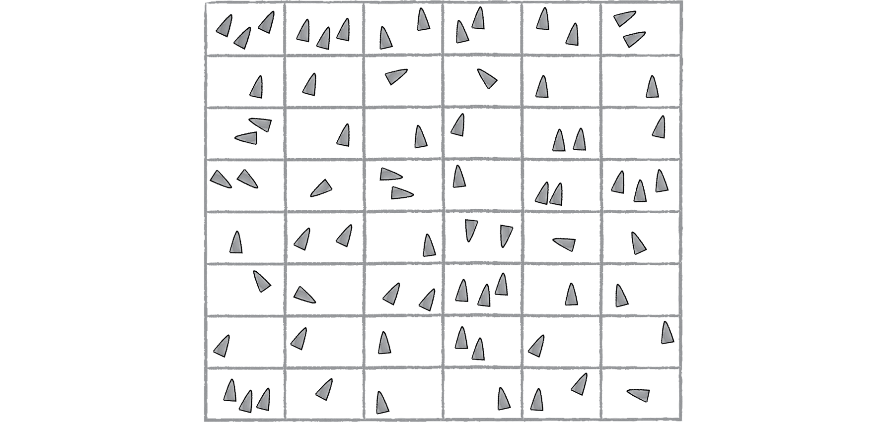
Figure 6.37

This technique is known as “bin-lattice spatial subdivision” and is outlined in more detail in (surprise, surprise) Reynolds’s 2000 paper, “Interaction with Groups of Autonomous Characters”. How do we implement such an algorithm in Processing? One way is to keep multiple ArrayLists. One ArrayList would keep track of all the boids, just like in our flocking example.

ArrayList<Boid> boids;

In addition to that ArrayList, we store an additional reference to each Boid object in a two-dimensional ArrayList. For each cell in the grid, there is an ArrayList that tracks the objects in that cell.

ArrayList<Boid>[][] grid;

In the main draw() loop, each Boid object then registers itself in the appropriate cell according to its location.

int column = int(boid.x) / resolution;
int row    = int(boid.y) /resolution;
grid[column][row].add(boid);

Then when it comes time to have the boids check for neighbors, they can look at only those in their particular cell (in truth, we also need to check neighboring cells to deal with border cases).

Example 6.10: Bin-lattice spatial subdivision

int column = int(boid.x) / resolution;
int row    = int(boid.y) /resolution;
boid.flock(boids);

boid.flock(grid[column][row]);

We’re only covering the basics here; for the full code, check the book’s website.

Now, there are certainly flaws with this system. What if all the boids congregate in the corner and live in the same cell? Then don’t we have to check all 2,000 against all 2,000?

The good news is that this need for optimization is a common one and there are a wide variety of similar techniques out there. For us, it’s likely that a basic approach will be good enough (in most cases, you won’t need one at all.) For another, more sophisticated approach, check out toxiclibs' Octree examples.

6.15 A Few Last Notes: Optimization Tricks

This is something of a momentous occasion. The end of Chapter 6 marks the end of our story of motion (in the context of this book, that is). We started with the concept of a vector, moved on to forces, designed systems of many elements, examined physics libraries, built entities with hopes and dreams and fears, and simulated emergence. The story doesn’t end here, but it does take a bit of a turn. The next two chapters won’t focus on moving bodies, but rather on systems of rules. Before we get there, I have a few quick items I’d like to mention that are important when working with the examples in Chapters 1 through 6. They also relate to optimizing your code, which fits in with the previous section.

float mag() {
  return sqrt(x*x + y*y);
}

if (v.mag() > 10) {
  // Do Something!
}

if (v.magSq() > 100) {
  // Do Something!
}

float magSq() {
  return x*x + y*y;
}

void draw() {
  for (int i = 0; i < 10000; i++) {
     println(sin(PI));
  }
}

float sinvalues[] = new float[360];
float cosvalues[] = new float[360];
for (int i = 0; i < 360; i++) {
  sinvalues[i] = sin(radians(i));
  cosvalues[i] = cos(radians(i));
}

int angle = int(degrees(PI));
float answer = sinvalues[angle];

void draw() {
  for (Vehicle v : vehicles) {
   PVector mouse = new PVector(mouseX,mouseY);
   v.seek(mouse);
  }
}

void draw() {
  PVector mouse = new PVector(mouseX,mouseY);
  for (Vehicle v : vehicles) {
   v.seek(mouse);
  }
}

PVector mouse = new PVector();
 
void draw() {
  mouse.x = mouseX;
  mouse.y = mouseY;
  for (Vehicle v : vehicles) {
   v.seek(mouse);
  }
}

    PVector desired = PVector.sub(target,location);
    desired.normalize();
    desired.mult(maxspeed);
 

    PVector steer = PVector.sub(desired,velocity);
    steer.limit(maxforce);
    return steer;

    PVector desired = PVector.sub(target, location);
    desired.normalize();
    desired.mult(maxspeed);
 

    desired.sub(velocity);
    desired.limit(maxforce);
    return desired;