5.1 What Is Box2D and When Is It Useful?

Box2D began as a set of physics tutorials written in C++ by Erin Catto for the Game Developer’s Conference in 2006. Over the last five years it has evolved into an rich and elaborate open-source physics engine. It’s been used for countless projects, most notably highly successful games such as the award-winning puzzle game Crayon Physics and the runaway mobile and tablet hit Angry Birds.

One of the key things to realize about Box2D is that it is a true physics engine. Box2D knows nothing about computer graphics and the world of pixels; it is simply a library that takes in numbers and spits out more numbers. And what are those numbers? Meters, kilograms, seconds, etc. All of Box2D’s measurements and calculations are for real-world measurements—only its “world” is a two-dimensional plane with top, bottom, left, and right edges. You tell it things like: “The gravity of our world is 9.81 newtons per kilogram, and a circle with a radius of four meters and a mass of fifty kilograms is located ten meters above the world’s bottom.” Box2D will then tell you things like: “One second later, the rectangle is at five meters from the bottom; two seconds later, it is ten meters below,” etc. While this provides for an amazing and realistic physics engine, it also necessitates lots of complicated code in order to translate back and forth between the physics “world” (a key term in Box2D) and the world we want to draw on —the “pixel” world of Processing.

So when is it worth it to have this additional overhead? If I just want to simulate a circle falling down a Processing window with gravity, do I really need to write all the extra Box2D code just to get that effect? Certainly, the answer is no. We saw how to do this rather easily in the first chapter of this book. Let’s consider another scenario. What if I want to have a hundred of those circles falling? And what if those circles aren’t circles at all, but irregularly shaped polygons? And what if I want these polygons to bounce off each other in a realistic manner when they collide?

You may have noticed that the first four chapters of this book, while covering motion and forces in detail, has skipped over a rather important aspect of physics simulation—collisions. Let’s pretend for a moment that you aren’t reading a chapter about libraries and that we decided right now to cover how to handle collisions in a particle system. We’d have to evaluate and learn two distinct algorithms that address these questions:

If we’re thinking about shapes like rectangles or circles, question #1 isn’t too tough. You’ve likely encountered this before. For example, we know two circles are intersecting if the distance between them is less than the sum of their radii.

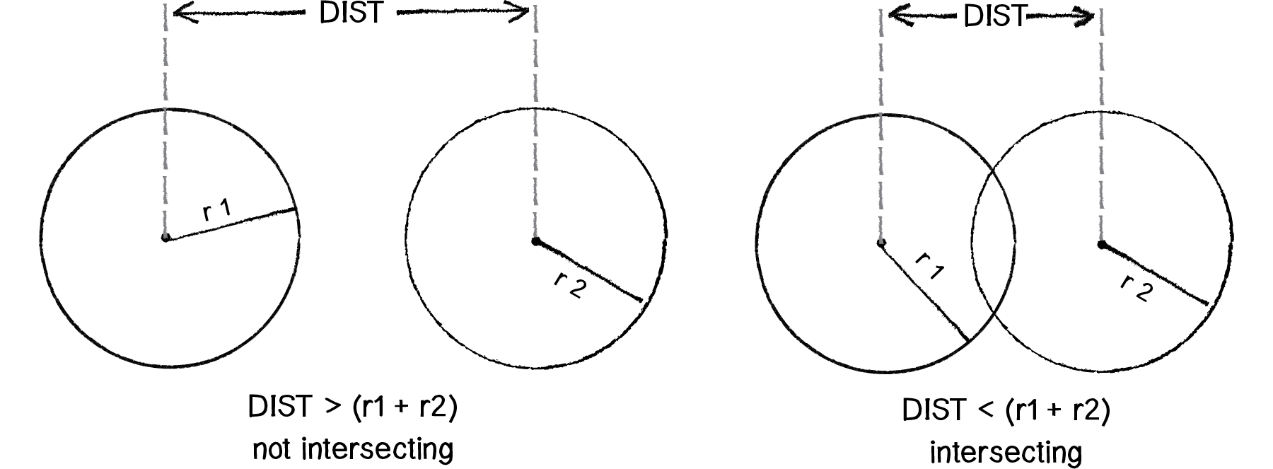
Figure 5.1

OK. Now that we know how to determine if two circles are colliding, how do we calculate their velocities after the collision? This is where we’re going to stop our discussion. Why, you ask? It’s not that understanding the math behind collisions isn’t important or valuable. (In fact, I’m including additional examples on the website related to collisions without a physics library.) The reason for stopping is that life is short (let this also be a reason for you to consider going outside and frolicking instead of programming altogether). We can’t expect to master every detail of physics simulation. And while we could continue this discussion for circles, it’s only going to lead us to wanting to work with rectangles. And strangely shaped polygons. And curved surfaces. And swinging pendulums colliding with springy springs. And and and and and.

Working with collisions in our Processing sketch while still having time to spend with our friends and family—that’s the reason for this chapter. Erin Catto spent years developing solutions to these kinds of problems so you don’t need to engineer them yourselves, at least for now.

In conclusion, if you find yourself describing an idea for a Processing sketch and the word “collisions” comes up, then it’s likely time to learn Box2D. (We’ll also encounter other words that might lead you down this path to Box2D, such as “joint,” “hinge,” “pulley,” “motor,” etc.)

5.2 Getting Box2D in Processing

So, if Box2D is a physics engine that knows nothing about pixel-based computer graphics and is written in C++, how are we supposed to use it in Processing?

The good news is that Box2D is such an amazing and useful library that everyone wants to use it—Flash, Javascript, Python, Ruby programmers. Oh, and Java programmers. There is something called JBox2D, a Java port of Box2D. And because Processing is built on top of Java, JBox2D can be used directly in Processing!

So here’s where we are so far.

This is all you need to get started writing Box2D code in Processing. However, as we are going to see in a moment, there are several pieces of functionality we’ll repeatedly need in our Processing code, and so it’s worth having one additional layer between our sketches and JBox2D. I’m calling this PBox2D—a Processing Box2D “helper” library included as part of this book’s code example downloads.

It’s important to realize that PBox2D is not a Processing wrapper for all of Box2D. After all, Box2D is a thoughtfully organized and well-structured API and there’s no reason to take it apart and re-implement it. However, it’s useful to have a small set of functions that help you get your Box2D world set up, as well as help you figure out where to draw your Box2D shapes. And this is what PBox2D will provide.

I should also mention before we move forward that there are other Processing libraries that wrap Box2D for you. One I would recommend taking a look at is Fisica by Ricard Marxer.

5.3 Box2D Basics

Do not despair! We really are going to get to the code very soon, and in some ways we’ll blow our previous work out of the water. But before we’re ready to do that, it’s important to walk through the overall process of using Box2D in Processing. Let’s begin by writing a pseudocode generalization of all of our examples in Chapters 1 through 4.

SETUP:

DRAW:

Great. Let’s rewrite this pseudocode as it will appear in our Box2D examples.

SETUP:

DRAW:

This, of course, is the fantasy of Box2D. We’ve eliminated all of those painful steps of figuring out how the objects are moving according to velocity and acceleration. Box2D is going to take care of this for us! The good news is that this does accurately reflect the overall process. Let’s imagine Box2D as a magic box.

In setup(), we’re going to say to Box2D: “Hello there. Here are all of the things I want in my world.” In draw(), we’re going to politely ask Box2D: “Oh, hello again. If it’s not too much trouble, I’d like to draw all of those things in my world. Could you tell me where they are?”

The bad news: it’s not as simple as the above explanation would lead you to believe. For one, making the stuff that goes in the Box2D world involves wading through the documentation for how different kinds of shapes are built and configured. Second, we have to remember that we can’t tell Box2D anything about pixels, as it will simply get confused and fall apart. Before we tell Box2D what we want in our world, we have to convert our pixel units to Box2D “world” units. And the same is true when it comes time to draw our stuff. Box2D is going to tell us the location of the things in its world, which we then have to translate for the pixel world.

Now that we understand that anything we create in our Processing sketch has to be placed into the Box2D world, let’s look at an overview of the elements that make up that world.

In the next four sections, we are going to walk through each of the above elements in detail, building several examples along the way. But first there is one other important element we should briefly discuss.

          6.   Vec2: Describes a vector in the Box2D world.

And so here we are, arriving with trepidation at an unfortunate truth in the world of using physics libraries. Any physics simulation is going to involve the concept of a vector. This is the good part. After all, we just spent several chapters familiarizing ourselves with what it means to describe motion and forces with vectors. We don’t have to learn anything new conceptually.

Now for the part that makes the single tear fall from my eye: we don’t get to use PVector. It’s nice that Processing has PVector for us, but anytime you use a physics library you will probably discover that the library includes its own vector implementation. This makes sense, after all; why should Box2D be expected to know about PVector? And in many cases, the physics engine will want to implement a vector class in a specific way so that it is especially compatible with the rest of the library’s code. So while we don’t have to learn anything new conceptually, we do have to get used to some new naming conventions and syntax. Let’s quickly demonstrate a few of the basics in Vec2 as compared to those in PVector.

Let’s say we want to add two vectors together.

PVector a = new PVector(1,-1);
PVector b = new PVector(3,4);
a.add(b);

Vec2 a = new Vec2(1,-1);
Vec2 b = new Vec2(3,4);
a.addLocal(b);

PVector a = new PVector(1,-1);
PVector b = new PVector(3,4);
PVector c = PVector.add(a,b);

Vec2 a = new Vec2(1,-1);
Vec2 b = new Vec2(3,4);
Vec2 c = a.add(b);

How about if we want to multiply and scale them?

PVector a = new PVector(1,-1);
float n = 5;
a.mult(n);

Vec2 a = new Vec2(1,-1);
float n = 5;
a.mulLocal(n);

PVector a = new PVector(1,-1);
float n = 5;
PVector c = PVector.mult(a,n);

Vec2 a = new Vec2(1,-1);
float n = 5;
Vec2 c = a.mul(n);

Magnitude and normalize?

PVector a = new PVector(1,-1);
float m = a.mag();
a.normalize();

Vec2 a = new Vec2(1,-1);
float m = a.length();
a.normalize();

As you can see, the concepts are the same, but the function names and the arguments are slightly different. For example, instead of static and non-static add() and mult(), if a Vec2 is altered, the word “local” is included in the function name—addLocal(), multLocal().

We’ll cover the basics of what you need to know here, but if you are looking for more, full documentation of Vec2 can be found by downloading the JBox2D source code.

5.4 Living in a Box2D World

The Box2D World object is in charge of everything. It manages the coordinate space of the world, all of the stuff that lives in the world, and decides when time moves forward in the world.

In order to have Box2D as part of our Processing sketches, the World is the very first thing that needs to be set up. Here is where PBox2D comes in handy and takes care of making the world for us.

PBox2D box2d;
 
void setup() {
  box2d = new PBox2D(this);

  box2d.createWorld();
}

When you call createWorld(), PBox2D will set up a default gravity for you (pointing down); however, you can always alter the gravity of your world by saying:

  box2d.setGravity(0, -10);

It’s worth noting that gravity doesn’t have to be fixed, nor does it always have to point downwards; you can adjust the gravity vector while your program is running. Gravity can be turned off by setting it to a (0,0) vector.

So, what are those numbers 0 and -10? This should remind us of one of the most important details of using Box2D: the Box2D coordinate system is not your pixel coordinate system! Let’s look at how Box2D and a Processing window think differently of their worlds.

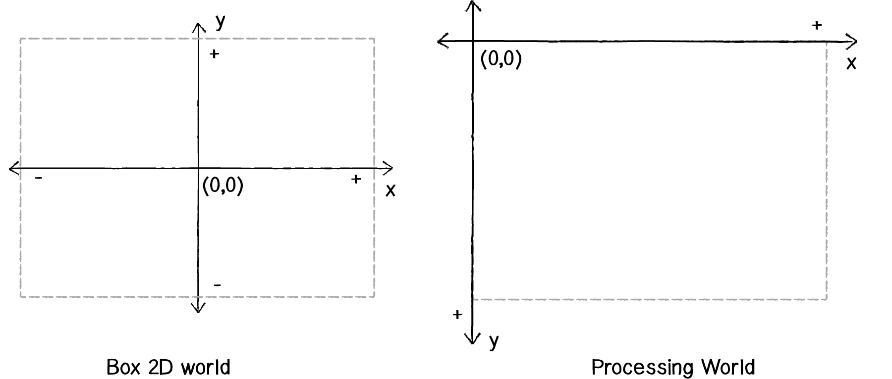
Figure 5.2

Notice how in Box2D (0,0) is in the center and up is the positive direction along the y-axis! Box2D’s coordinate system is just like that lovely old-fashioned Cartesian one with (0,0) in the center and up pointing in a positive direction. Processing, on the other hand, uses a traditional computer graphics coordinate system where (0,0) is in the top left corner and down is the positive direction along the y-axis. This is why if we want objects to fall down with gravity, we need to give Box2D a gravity force with a negative y-value.

Vec2 gravity = new Vec2(0, -10);

Luckily for us, if we prefer to think in terms of pixel coordinates (which as Processing programmers, we are likely to do), PBox2D offers a series of helper functions that convert between pixel space and Box2D space. Before we move onto the next section and begin creating Box2D bodies, let’s take a look at how these helper functions work.

Let’s say we want to tell Box2D where the mouse is in its world. We know the mouse is located at (mouseX,mouseY) in Processing. To convert it, we say we want to convert a “coordinate” from “pixels” to “world”—coordPixelsToWorld(). Or:

Vec2 mouseWorld = box2d.coordPixelsToWorld(mouseX,mouseY);

What if we had a Box2D world coordinate and wanted to translate it to our pixel space?

Vec2 worldPos = new Vec2(-10,25);
 

Vec2 pixelPos = box2d.coordWorldToPixels(worldPos);
ellipse(pixelPos.x, pixelPos.y,16,16);

PBox2D has a set of functions to take care of translating back and forth between the Box2D world and pixels. It’s probably easier to learn about all of these functions during the course of actually implementing our examples, but let’s quickly look over the list of the possibilities.

Vec2 coordWorldToPixels(Vec2 world)

Vec2 coordWorldToPixels(float worldX, float worldY)

Vec2 coordPixelsToWorld(Vec2 screen)

Vec2 coordPixelsToWorld(float pixelX, float pixelY)

float scalarPixelsToWorld(float val)

float scalarWorldToPixels(float val)

There are also additional functions that allow you to pass or receive a PVector when translating back and forth, but since we are only working with Box2D in the examples in this chapter, it’s easiest to stick with the Vec2 class for all vectors.

Once the world is initialized, we are ready to actually put stuff in the world—Box2D bodies.

5.5 Building a Box2D Body

A Box2D body is the primary element in the Box2D world. It’s the equivalent to the Mover class we built on our own in previous chapters—the thing that moves around the space and experiences forces. It can also be static (meaning fixed and not moving). It’s important to note, however, that a body has no geometry; it isn’t anything physical. Rather, bodies have Box2D shapes attached to them. (This way, a body can be a single rectangle or a rectangle attached to a circle, etc.) We’ll look at shapes in a moment; first, let’s build a body.

BodyDef bd = new BodyDef();

Vec2 center = new Vec2(width/2,height/2);

Vec2 center = box2d.coordPixelsToWorld(width/2,height/2));

bd.position.set(center);

bd.fixedRotation = true;

bd.linearDamping = 0.8;
bd.angularDamping = 0.9;

bd.bullet = true;

Body body = box2d.createBody(bd);

body.setLinearVelocity(new Vec2(0,3));

body.setAngularVelocity(1.2);

5.6 Three’s Company: Bodies and Shapes and Fixtures

A body on its own doesn’t physically exist in the world. It’s like a soul with no human form to inhabit. For a body to have mass, we must first define a shape and attach that shape to the body with something known as a fixture.

The job of the Box2D Shape class is to keep track of all the necessary collision geometry attached to a body. A shape also has several important properties that affect the body’s motion. There is density, which ultimately determines that body’s mass. Shapes also have friction and restitution (“bounciness”) which will be defined through a fixture. One of the nice things about Box2D’s methodology, which separates the concepts of bodies and shapes into two separate objects, is that you can attach multiple shapes to a single body in order to create more complex forms. We’ll see this in a future example.

To create a shape, we need to first decide what kind of shape we want to make. For most non-circular shapes, a PolygonShape object will work just fine. For example, let’s look at how we define a rectangle.

PolygonShape ps = new PolygonShape();

float box2Dw = box2d.scalarPixelsToWorld(150);
float box2Dh = box2d.scalarPixelsToWorld(100);

ps.setAsBox(box2Dw, box2Dh);

FixtureDef fd = new FixtureDef();

fd.shape = ps;

fd.friction = 0.3;

fd.restitution = 0.5;

fd.density = 1.0;

body.createFixture(fd);

body.createFixture(ps,1);

BodyDef bd = new BodyDef();
bd.position.set(box2d.coordPixelsToWorld(width/2,height/2));
 

Body body = box2d.createBody(bd);
 

PolygonShape ps = new PolygonShape();
float w = box2d.scalarPixelsToWorld(150);
float h = box2d.scalarPixelsToWorld(100);
ps.setAsBox(w, h);
 

FixtureDef fd = new FixtureDef();
fd.shape = ps;
fd.density = 1;
fd.friction = 0.3;
fd.restitution = 0.5;
 

body.createFixture(fd);

CircleShape cs = new CircleShape();
float radius = 10;
cs.m_radius = ____________________;
FixtureDef fd = new FixtureDef();
fd.shape = cs;
fd.density = 1;
fd.friction = 0.1;
fd.restitution = 0.3;
 
body.createFixture(fd);

5.7 Box2D and Processing: Reunited and It Feels So Good

Once a body is made, it lives in the Box2D physics world. Box2D will always know it’s there, check it for collisions, move it appropriately according to the forces, etc. It’ll do all that for you without you having to lift a finger! What it won’t do, however, is display the body for you. This is a good thing. This is your time to shine. When working with Box2D, what we’re essentially saying is, “I want to be the designer of my world, and I want you, Box2D, to compute all the physics.”

Now, Box2D will keep a list of all the bodies that exist in the world. This can be accessed by calling the World object’s getBodyList() function. Nevertheless, what I’m going to demonstrate here is a technique for keeping your own body lists. Yes, this may be a bit redundant and we perhaps sacrifice a bit of efficiency. But we more than make up for that with ease of use. This methodology will allow us to program like we’re used to in Processing, and we can easily keep track of which bodies are which and render them appropriately. Let’s consider the structure of the following Processing sketch:

Figure 5.3

This looks like any ol’ Processing sketch. We have a main tab called “Boxes” and a “Boundary” and a “Box” tab. Let’s think about the Box tab for a moment. The Box tab is where we will write a simple class to describe a Box object, a rectangular body in our world.

class Box  {
 

  float x,y;
  float w,h;

 
  Box(float x_, float y_) {

    x = x_;
    y = y_;

    w = 16;
    h = 16;
  }
 
  void display() {

    fill(175);
    stroke(0);
    rectMode(CENTER);
    rect(x,y,w,h);
  }
}

Let’s write a main tab that creates a new Box whenever the mouse is pressed and stores all the Box objects in an ArrayList. (This is very similar to our approach in the particle system examples from Chapter 4.)

Example 5.1: A comfortable and cozy Processing sketch that needs a little Box2D

ArrayList<Box> boxes;
 
void setup() {
  size(400,300);
  boxes = new ArrayList<Box>();
}
 
void draw() {
  background(255);
 

  if (mousePressed) {
    Box p = new Box(mouseX,mouseY);
    boxes.add(p);
  }

  for (Box b: boxes) {
    b.display();
  }

}

Now, here’s our assignment. Take the above example verbatim, but instead of drawing fixed boxes on the screen, draw boxes that experience physics (via Box2D) as soon as they appear.

We’ll need two major steps to accomplish our goal.

PBox2D box2d;
 
void setup() {

  box2d = new PBox2D(this);
  box2d.createWorld();

}

void draw() {

  box2d.step();
}

Step 2: Link every Processing Box object with a Box2D Body object.

As of this moment, the Box class includes variables for location and width and height. What we now want to say is:

“I hereby relinquish the command of this object’s position to Box2D. I no longer need to keep track of anything related to location, velocity, and acceleration. Instead, I only need to keep track of a Box2D body and have faith that Box2D will do the rest.”

Show Raw class Box { // Instead of any of the usual variables, // we will store a reference to a Box2D body. Body body; float w; float h;

class Box  {
 

Instead of any of the usual variables, we will store a reference to a Box2D body.

  Body body;
  float w;
  float h;

We don’t need (x,y) anymore since, as we’ll see, the body itself will keep track of its location. The body technically could also keep track of the width and height for us, but since Box2D isn’t going to do anything to alter those values over the life of the Box object, we might as well just hold onto them ourselves until it’s time to draw the Box.

Then, in our constructor, in addition to initializing the width and height, we can go ahead and include all of the body and shape code we learned in the previous two sections!

Show Raw Box() { w = 16; h = 16; // Build body. BodyDef bd = new BodyDef(); bd.type = BodyType.DYNAMIC; bd.position.set(box2d.coordPixelsToWorld(mouseX,mouseY)); body = box2d.createBody(bd); // Build shape. PolygonShape ps = new PolygonShape(); //[full] Box2D considers the width and height of a rectangle to be the distance from the center to the edge (so half of what we normally think of as width or height). float box2dW = box2d.scalarPixelsToWorld(w/2); float box2dH = box2d.scalarPixelsToWorld(h/2); //[end] ps.setAsBox(box2dW, box2dH); FixtureDef fd = new FixtureDef(); fd.shape = ps; fd.density = 1; // Set physics parameters. fd.friction = 0.3; fd.restitution = 0.5; // Attach the Shape to the Body with the Fixture. body.createFixture(fd); }

  Box() {
    w = 16;
    h = 16;
 

Build body.

    BodyDef bd = new BodyDef();
    bd.type = BodyType.DYNAMIC;
    bd.position.set(box2d.coordPixelsToWorld(mouseX,mouseY));
    body = box2d.createBody(bd);
 

Build shape.

    PolygonShape ps = new PolygonShape();

Box2D considers the width and height of a rectangle to be the distance from the center to the edge (so half of what we normally think of as width or height).

    float box2dW = box2d.scalarPixelsToWorld(w/2);
    float box2dH = box2d.scalarPixelsToWorld(h/2);

    ps.setAsBox(box2dW, box2dH);
 
    FixtureDef fd = new FixtureDef();
    fd.shape = ps;
    fd.density = 1;

Set physics parameters.

    fd.friction = 0.3;
    fd.restitution = 0.5;
 

Attach the Shape to the Body with the Fixture.

    body.createFixture(fd);
 }

OK, we’re almost there. Before we introduced Box2D, it was easy to draw the Box. The object’s location was stored in variables x and y.

Show Raw //[full] Drawing the object using rect() void display() { fill(175); stroke(0); rectMode(CENTER); rect(x,y,w,h); } //[end]

Drawing the object using rect()

  void display() {
    fill(175);
    stroke(0);
    rectMode(CENTER);
    rect(x,y,w,h);
  }

But now Box2D manages the object’s motion, so we can no longer use our own variables to display the shape. Not to fear! Our Box object has a reference to the Box2D body associated with it. So all we need to do is politely ask the body, “Pardon me, where are you located?” Since this is a task we’ll need to do quite often, PBox2D includes a helper function: getBodyPixelCoord().

Show Raw Vec2 pos = box2d.getBodyPixelCoord(body);

Vec2 pos = box2d.getBodyPixelCoord(body);

Just knowing the location of a body isn’t enough; we also need to know its angle of rotation.

Show Raw float a = body.getAngle();

float a = body.getAngle();

Once we have the location and angle, it’s easy to display the object using translate() and rotate(). Note, however, that the Box2D coordinate system considers rotation in the opposite direction from Processing, so we need to multiply the angle by -1.

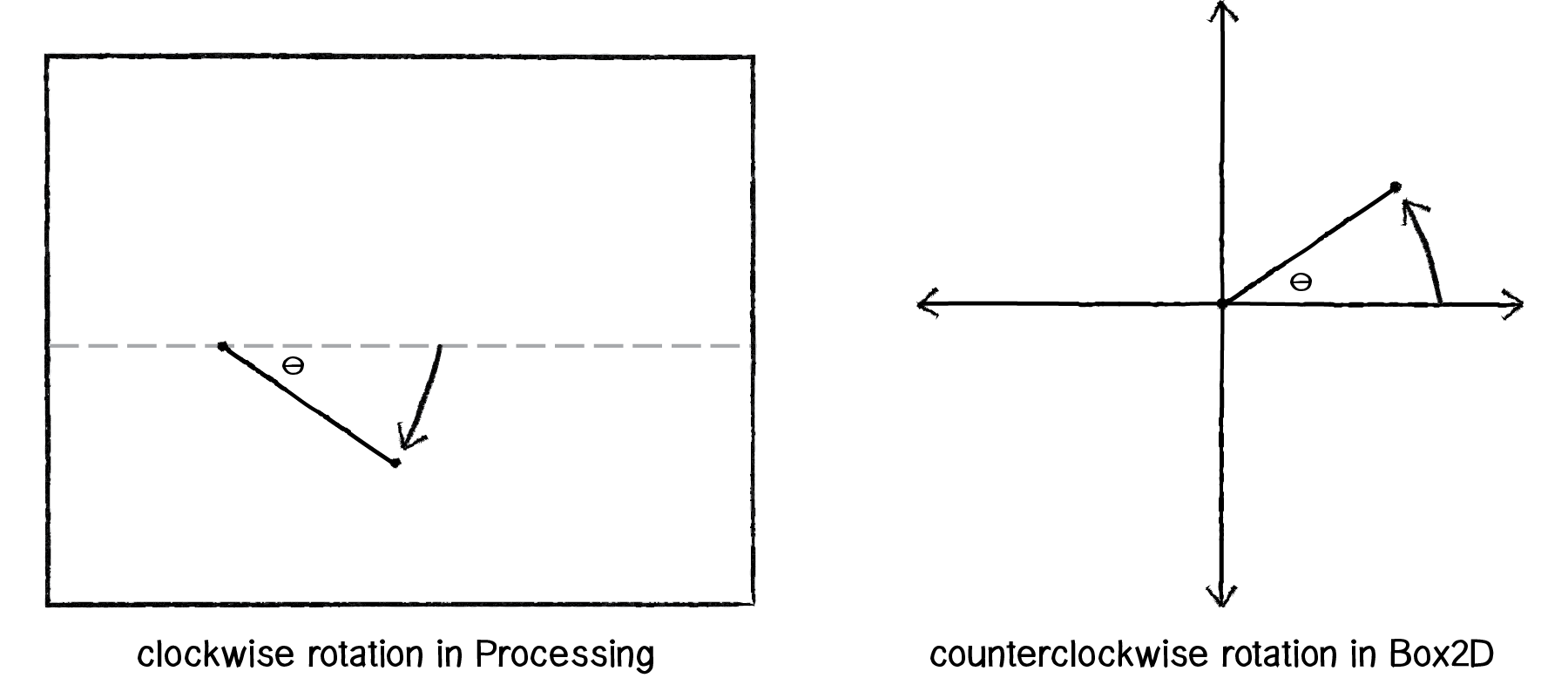
Figure 5.4

Show Raw void display() { //[full] We need the Body’s location and angle. Vec2 pos = box2d.getBodyPixelCoord(body); float a = body.getAngle(); //[end] pushMatrix(); //[full] Using the Vec2 position and float angle to translate and rotate the rectangle translate(pos.x,pos.y); rotate(-a); //[end] fill(175); stroke(0); rectMode(CENTER); rect(0,0,w,h); popMatrix(); }

  void display() {

We need the Body’s location and angle.

    Vec2 pos = box2d.getBodyPixelCoord(body);
    float a = body.getAngle();

 
    pushMatrix();

Using the Vec2 position and float angle to translate and rotate the rectangle

    translate(pos.x,pos.y);
    rotate(-a);

    fill(175);
    stroke(0);
    rectMode(CENTER);
    rect(0,0,w,h);
    popMatrix();
  }

In case we want to have objects that can be removed from the Box2D world, it’s also useful to include a function to destroy a body, such as:

Show Raw // This function removes a body from the Box2D world. void killBody() { box2d.destroyBody(body); }

This function removes a body from the Box2D world.

  void killBody() {
    box2d.destroyBody(body);
  }

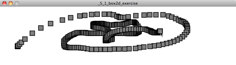
Exercise 5.2

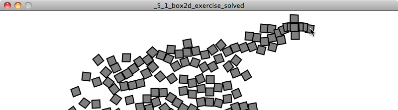
In this chapter’s code downloads, find the sketch named “box2d_exercise.” Using the methodology outlined in this chapter, add the necessary code to the main and Box tabs to implement Box2D physics. The result should appear as in the screenshot above. Be more creative in how you render the boxes.

5.8 Fixed Box2D Objects

In the example we just created, the Box objects appear at the mouse location and fall downwards due to Box2D’s default gravity force. What if we wanted to install some immovable boundaries in the Box2D world that would block the path of the Box objects (as in the illustration below)?

Box2D makes this easy for us by providing a means to lock a body (and any associated shapes) in place. Just set the BodyDef object’s type to STATIC.

 BodyDef bd = new BodyDef();

 bd.type = BodyType.STATIC;

We can add this feature to our Boxes example by writing a Boundary class and having each boundary create a fixed Box2D body.

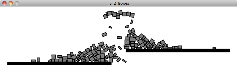
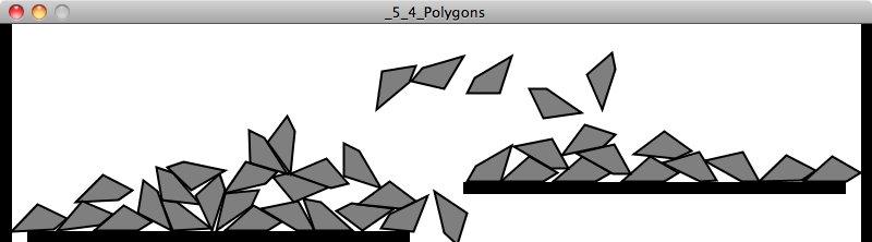
Example 5.2: Falling boxes hitting boundaries

class Boundary {
 

  float x,y;
  float w,h;

  Body b;
 
  Boundary(float x_,float y_, float w_, float h_) {
    x = x_;
    y = y_;
    w = w_;
    h = h_;
 

    BodyDef bd = new BodyDef();
    bd.position.set(box2d.coordPixelsToWorld(x,y));

    bd.type = BodyType.STATIC;
    b = box2d.createBody(bd);
 
    float box2dW = box2d.scalarPixelsToWorld(w/2);
    float box2dH = box2d.scalarPixelsToWorld(h/2);
    PolygonShape ps = new PolygonShape();

    ps.setAsBox(box2dW, box2dH);
 

    b.createFixture(ps,1);
  }
 

  void display() {
    fill(0);
    stroke(0);
    rectMode(CENTER);
    rect(x,y,w,h);
  }
 
}

5.9 A Curvy Boundary

If you want a fixed boundary that is a curved surface (as opposed to a polygon), this can be achieved with the shape ChainShape.

The ChainShape class is another shape like PolygonShape or CircleShape, so to include one in our system, we follow the same steps.

BodyDef bd = new BodyDef();
Body body = box2d.world.createBody(bd);

ChainShape chain = new ChainShape();

Step 3: Configure the Shape.

The ChainShape object is a series of connected vertices. To create the chain, we must first specify an array of vertices (each as a Vec2 object). For example, if we wanted a straight line from the left-hand side of our window to the right-hand side, we would just need an array of two vertices: (0,150) and (width,150). (Note that if you want to create a loop where the first vertex connects to the last vertex in a loop, you can use the ChainLoop class instead.)

Show Raw Vec2[] vertices = new Vec2[2]; // Adding a vertex on the right side of window vertices[0] = box2d.coordPixelsToWorld(0,150); // Adding a vertex on the left side of window vertices[1] = box2d.coordPixelsToWorld(width,150);

Vec2[] vertices = new Vec2[2];

Adding a vertex on the right side of window

vertices[0] = box2d.coordPixelsToWorld(0,150);

Adding a vertex on the left side of window

vertices[1] = box2d.coordPixelsToWorld(width,150);

To create the chain with the vertices, the array is then passed into a function called createChain().

Show Raw // If you don’t want to use the entire array, // you can specify a value less than length. chain.createChain(vertices, vertices.length);

If you don’t want to use the entire array, you can specify a value less than length.

chain.createChain(vertices, vertices.length);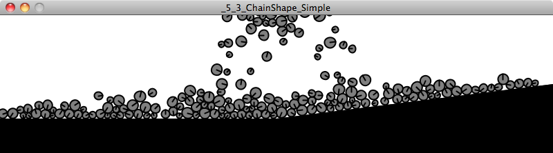

Step 4: Attach the Shape to the body with a Fixture.

A Shape is not part of Box2D unless it is attached to a body. Even if it is a fixed boundary and never moves, it must still be attached. Just as with other shapes, a ChainShape object can be given properties like restitution and friction with a Fixture.

Show Raw FixtureDef fd = new FixtureDef(); // A fixture assigned to the ChainShape fd.shape = chain; fd.density = 1; fd.friction = 0.3; fd.restitution = 0.5; body.createFixture(fd);

FixtureDef fd = new FixtureDef();

A fixture assigned to the ChainShape

fd.shape = chain;
fd.density = 1;
fd.friction = 0.3;
fd.restitution = 0.5;
 
body.createFixture(fd);

Now, if we want to include a ChainShape object in our sketch, we can follow the same strategy as we did with a fixed boundary. Let’s write a class called Surface:

Example 5.3: ChainShape with three hard-coded vertices

Show Raw class Surface { ArrayList<Vec2> surface; Surface() { surface = new ArrayList<Vec2>(); //[full] 3 vertices in pixel coordinates surface.add(new Vec2(0, height/2+50)); surface.add(new Vec2(width/2, height/2+50)); surface.add(new Vec2(width, height/2)); //[end] ChainShape chain = new ChainShape(); // Make an array of Vec2 for the ChainShape. Vec2[] vertices = new Vec2[surface.size()]; for (int i = 0; i < vertices.length; i++) { //[offset-up] Convert each vertex to Box2D World coordinates. vertices[i] = box2d.coordPixelsToWorld(surface.get(i)); } // Create the ChainShape with array of Vec2. chain.createChain(vertices, vertices.length); //[full] Attach the Shape to the Body. BodyDef bd = new BodyDef(); Body body = box2d.world.createBody(bd); body.createFixture(chain, 1); //[end] }

class Surface {
  ArrayList<Vec2> surface;
 
  Surface() {
 
    surface = new ArrayList<Vec2>();

3 vertices in pixel coordinates

    surface.add(new Vec2(0, height/2+50));
    surface.add(new Vec2(width/2, height/2+50));
    surface.add(new Vec2(width, height/2));

 
    ChainShape chain = new ChainShape();
 

Make an array of Vec2 for the ChainShape.

    Vec2[] vertices = new Vec2[surface.size()];
 
 
    for (int i = 0; i < vertices.length; i++) {

Convert each vertex to Box2D World coordinates.

      vertices[i] = box2d.coordPixelsToWorld(surface.get(i));
    }
 

Create the ChainShape with array of Vec2.

    chain.createChain(vertices, vertices.length);
 

Attach the Shape to the Body.

    BodyDef bd = new BodyDef();
    Body body = box2d.world.createBody(bd);
    body.createFixture(chain, 1);

  }

Notice how the above class includes an ArrayList to store a series of Vec2 objects. Even though we fully intend to store the coordinates of the chain in the chain shape itself, we are choosing the ease of redundancy and keeping our own list of those points as well. Later, when we go to draw the Surface object, we don’t have to ask Box2D for the locations of the chain shape’s vertices.

Show Raw void display() { strokeWeight(1); stroke(0); noFill(); //[full] Draw the ChainShape as a series of vertices. beginShape(); for (Vec2 v: surface) { vertex(v.x,v.y); } //[end] endShape(); } }

  void display() {
    strokeWeight(1);
    stroke(0);
    noFill();

Draw the ChainShape as a series of vertices.

    beginShape();
    for (Vec2 v: surface) {
      vertex(v.x,v.y);
    }

    endShape();
  }
}

What we need in setup() and draw() for the Surface object is quite simple, given that Box2D takes care of all of the physics for us.

Show Raw PBox2D box2d; Surface surface; void setup() { size(500,300); box2d = new PBox2D(this); box2d.createWorld(); // Make a Surface object. surface = new Surface(); } void draw() { box2d.step(); background(255); // Draw the Surface. surface.display(); }

PBox2D box2d;
 
Surface surface;
 
void setup() {
  size(500,300);
  box2d = new PBox2D(this);
  box2d.createWorld();
 

Make a Surface object.

  surface = new Surface();
}
 
void draw() {
  box2d.step();
 
  background(255);

Draw the Surface.

  surface.display();
}

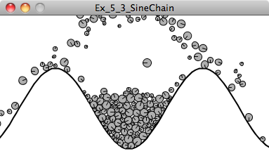
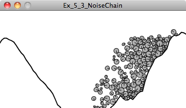
Exercise 5.3

Review how we learned to draw a wave pattern in Chapter 3. Create a ChainShape object out of a sine wave. Try using Perlin noise as well.

sine wave

Perlin noise

5.10 Complex Forms

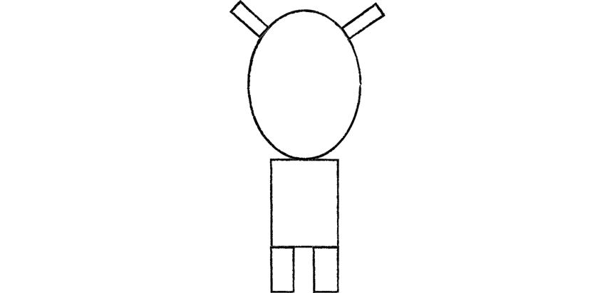
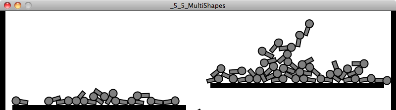
Figure 5.5

Now that we’ve seen how easy it is to make simple geometric forms in Box2D, let’s imagine that you want to have a more complex form, such as a little alien stick figure.

There are two strategies in Box2D for making forms that are more advanced than a basic circle or square. One is to use a PolygonShape in a different way. In our previous examples, we used PolygonShape to generate a rectangular shape with the setAsBox() function.

  PolygonShape ps = new PolygonShape();
  ps.setAsBox(box2dW, box2dH);

This was a good way to start because of the inherent simplicity of working with rectangles. However, a PolygonShape object can also be generated from an array of vectors, which allows you to build a completely custom shape as a series of connected vertices. This works very similarly to the ChainShape class.

Example 5.4: Polygon shapes

Vec2[] vertices = new Vec2[4];  // An array of 4 vectors
vertices[0] = box2d.vectorPixelsToWorld(new Vec2(-15, 25));
vertices[1] = box2d.vectorPixelsToWorld(new Vec2(15, 0));
vertices[2] = box2d.vectorPixelsToWorld(new Vec2(20, -15));
vertices[3] = box2d.vectorPixelsToWorld(new Vec2(-10, -10));
 

PolygonShape ps = new PolygonShape();
ps.set(vertices, vertices.length);

When building your own polygon in Box2D, you must remember two important details.

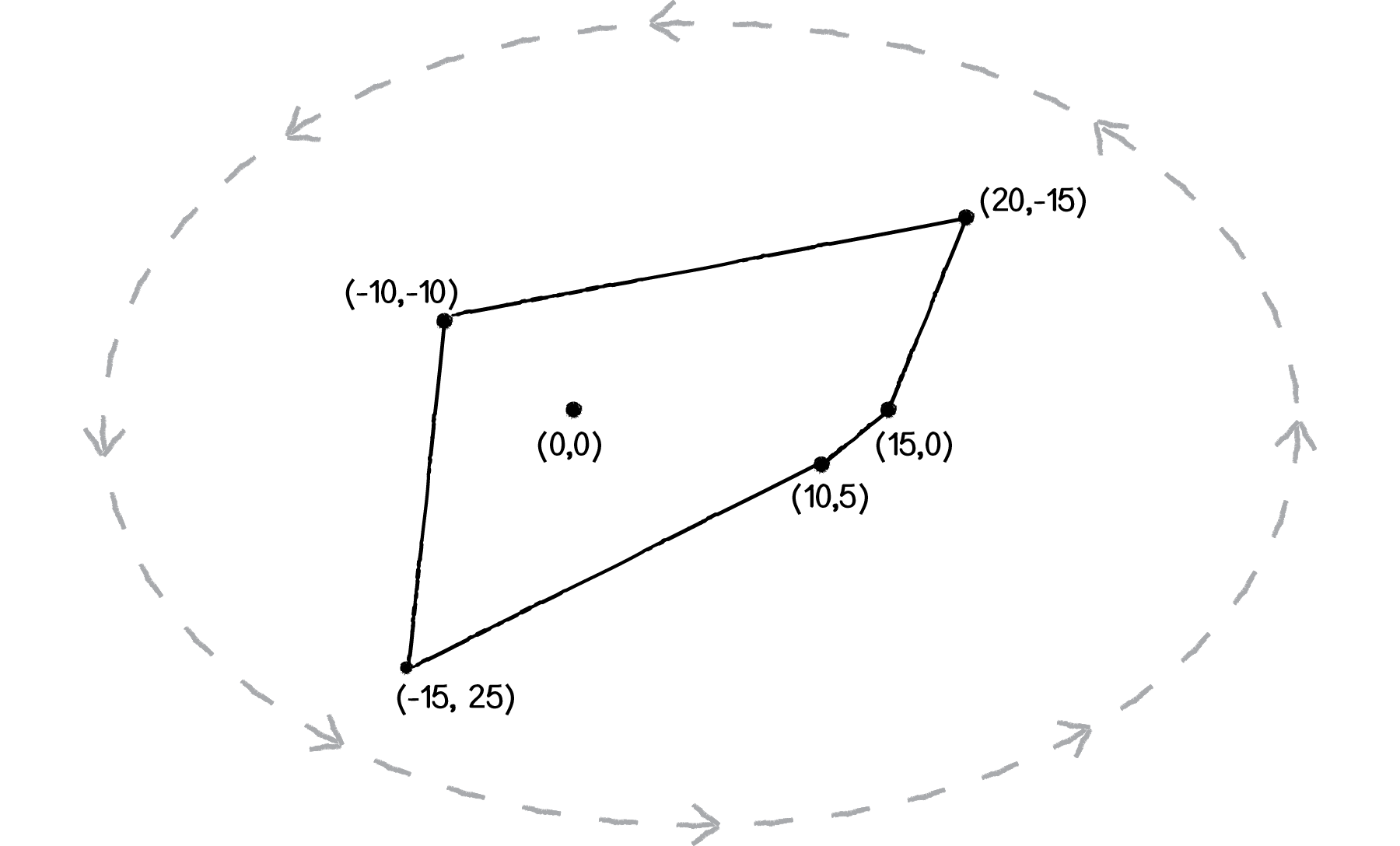
Figure 5.6

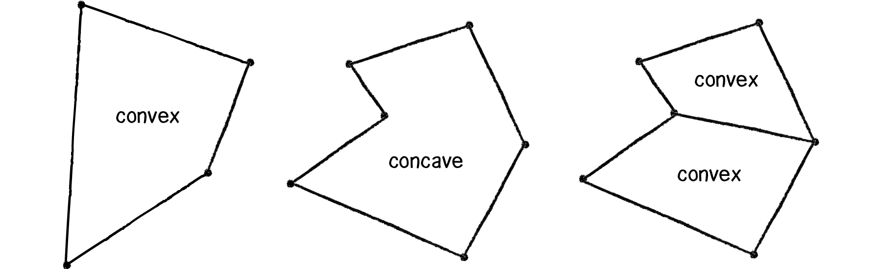
Figure 5.7: A concave shape can be drawn with multiple convex shapes.

Now, when it comes time to display the shape in Processing, we can no longer just use rect() or ellipse(). Since the shape is built out of custom vertices, we’ll want to use Processing’s beginShape(), endShape(), and vertex() functions. As we saw with the ChainShape, we could choose to store the pixel locations of the vertices in our own ArrayList for drawing. However, it’s also useful to see how we can ask Box2D to report back to use the vertex locations.

  void display() {
    Vec2 pos = box2d.getBodyPixelCoord(body);
    float a = body.getAngle();
 

    Fixture f = body.getFixtureList();

    PolygonShape ps = (PolygonShape) f.getShape();
 
    rectMode(CENTER);
    pushMatrix();
    translate(pos.x,pos.y);
    rotate(-a);
    fill(175);
    stroke(0);
    beginShape();

    for (int i = 0; i < ps.getVertexCount(); i++) {
      Vec2 v = box2d.vectorWorldToPixels(ps.getVertex(i));
      vertex(v.x,v.y);
    }
    endShape(CLOSE);
    popMatrix();
  }

Exercise 5.4

Using the PolygonShape class, create your own polygon design (remember, it must be concave). Some possibilities below.

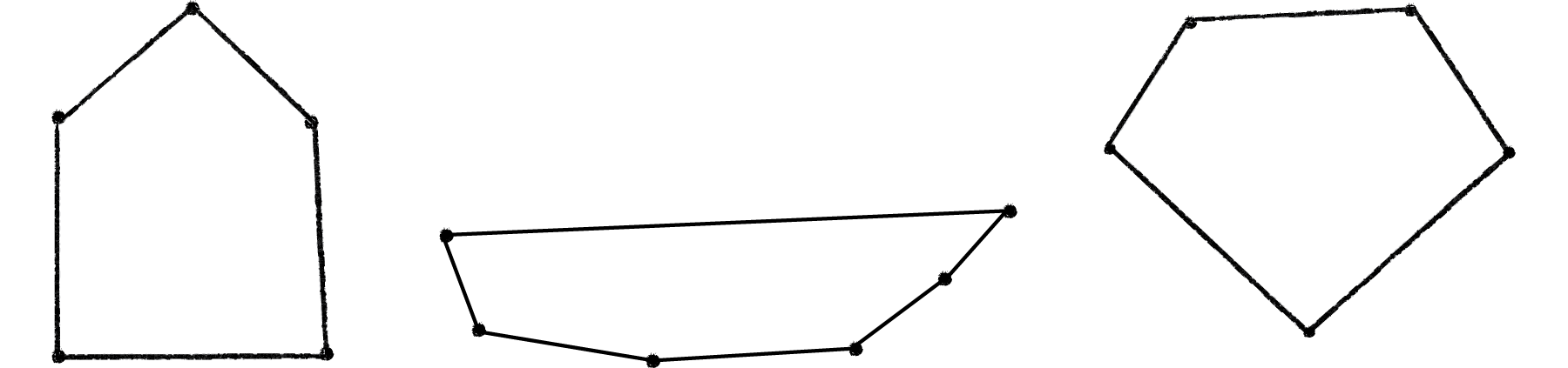
A polygon shape will get us pretty far in Box2D. Nevertheless, the convex shape requirement will severely limit the range of possibilities. The good news is that we can completely eliminate this restriction by creating a single Box2D body out of multiple shapes! Let’s return to our little alien creature and simplify the shape to be a thin rectangle with a circle on top.

How can we build a single body with two shapes? Let’s first review how we built a single body with one shape.

Step 1: Define the body.
Step 2: Create the body.
Step 3: Define the shape.
Step 4: Attach the shape to the body.
Step 5: Finalize the body’s mass.

Attaching more than one shape to a body is as simple as repeating steps 3 and 4 over and over again.

Step 3a: Define shape 1.
Step 4a: Attach shape 1 to the body.
Step 3b: Define shape 2.
Step 4b: Attach shape 2 to the body.
etc. etc. etc.

Let’s see what this would look like with actual Box2D code.

BodyDef bd = new BodyDef();
bd.type = BodyType.DYNAMIC;
bd.position.set(box2d.coordPixelsToWorld(center));
body = box2d.createBody(bd);

PolygonShape ps = new PolygonShape();
float box2dW = box2d.scalarPixelsToWorld(w/2);
float box2dH = box2d.scalarPixelsToWorld(h/2);
sd.setAsBox(box2dW, box2dH);

CircleShape cs = new CircleShape();
cs.m_radius = box2d.scalarPixelsToWorld(r);

body.createFixture(ps,1.0);
body.createFixture(cs, 1.0);

The above looks pretty good, but sadly, if we run it, we’ll get the following result:

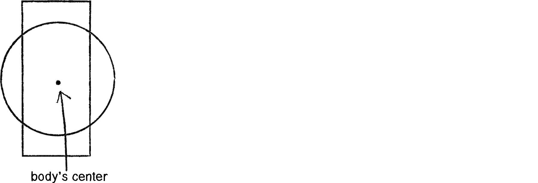
Figure 5.8

When you attach a shape to a body, by default, the center of the shape will be located at the center of the body. But in our case, if we take the center of the rectangle to be the center of the body, we want the center of the circle to be offset along the y-axis from the body’s center.

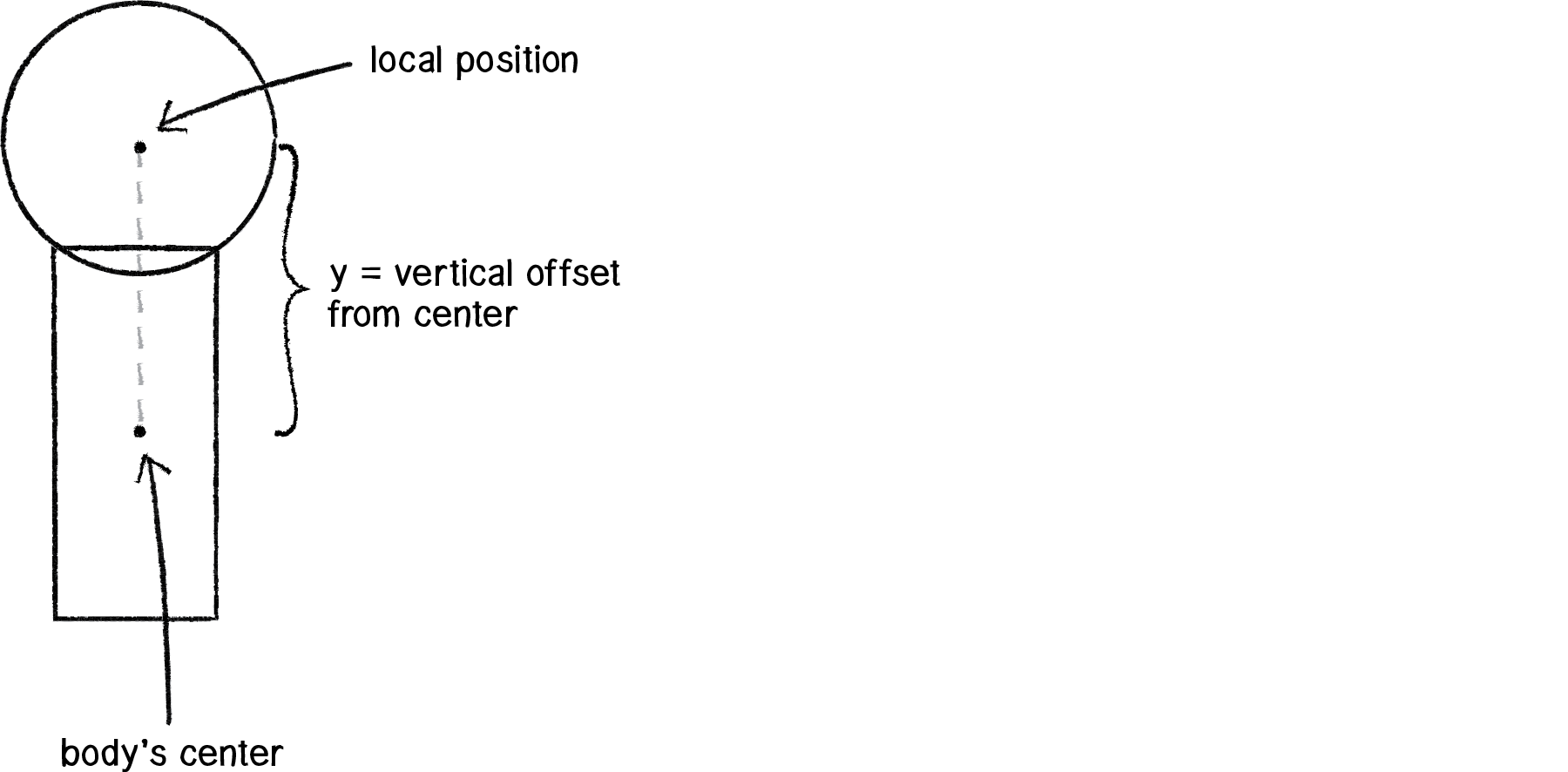
Figure 5.9

This is achieved by using the local position of a shape, accessed via a Vec2 variable called m_p.

Vec2 offset = new Vec2(0,-h/2);

offset = box2d.vectorPixelsToWorld(offset);

circle.m_p.set(offset.x,offset.y);

Then, when we go to draw the body, we use both rect() and ellipse() with the circle offset the same way.

Example 5.5: Multiple shapes on one body

  void display() {
    Vec2 pos = box2d.getBodyPixelCoord(body);
    float a = body.getAngle();
 
    rectMode(CENTER);
    pushMatrix();
    translate(pos.x,pos.y);
    rotate(-a);
    fill(175);
    stroke(0);

    rect(0,0,w,h);

    ellipse(0,-h/2,r*2,r*2);
    popMatrix();
  }

Finishing off this section, I want to stress the following: the stuff you draw in your Processing window doesn’t magically experience physics simply because we created some Box2D bodies and shapes. These examples work because we very carefully matched how we draw our elements with how we defined the bodies and shapes we put into the Box2D world. If you accidentally draw your shape differently, you won’t get an error, not from Processing or from Box2D. However, your sketch will look odd and the physics won’t work correctly. For example, what if we had written:

Vec2 offset = new Vec2(0,-h/2);

when we created the shape, but:

ellipse(0,h/2,r*2,r*2);

when it came time to display the shape?

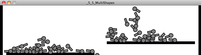
The results would look like the image above, where clearly, the collisions are not functioning as expected. This is not because the physics is broken; it’s because we did not communicate properly with Box2D, either when we put stuff in the magic world or queried the world for locations.

5.11 Feeling Attached—Box2D Joints

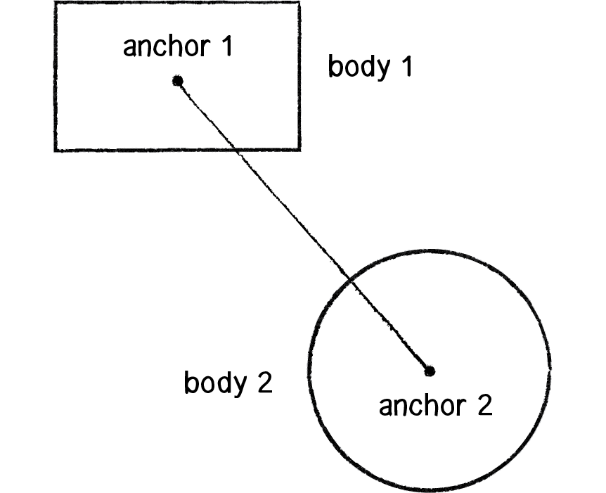
Figure 5.10

Box2D joints allow you to connect one body to another, enabling more advanced simulations of swinging pendulums, elastic bridges, squishy characters, wheels spinning on an axle, etc. There are many different kinds of Box2D joints. In this chapter we’re going to look at three: distance joints, revolute joints, and “mouse” joints.

Let’s begin with a distance joint, a joint that connects two bodies with a fixed length. The joint is attached to each body at a specified anchor point (a point relative to the body’s center). For any Box2D joint, we need to follow these steps. This, of course, is similar to the methodology we used to build bodies and shapes, with some quirks.

Step 1. Make sure you have two bodies ready to go.
Step 2. Define the joint.
Step 3. Configure the joint’s properties (What are the bodies? Where are the anchors? What is its rest length? Is it elastic or rigid?)
Step 4. Create the joint.

Let’s assume we have two Particle objects that each store a reference to a Box2D Body object. We’ll call them particles p1 and p2.

Particle p1 = new Particle();
Particle p2 = new Particle();

OK, onto Step 2. Let’s define the joint.

DistanceJointDef djd = new DistanceJointDef();

Easy, right? Now it’s time to configure the joint. First we tell the joint which two bodies it connects:

djd.bodyA = p1.body;
djd.bodyB = p2.body;

Then we set up a rest length. Remember, if our rest length is in pixels, we need to convert it!

djd.length = box2d.scalarPixelsToWorld(10);

A distance joint also includes two optional settings that can make the joint soft, like a spring connection: frequencyHz and dampingRatio.

  djd.frequencyHz  = ___;

  djd.dampingRatio = ___;

Finally, we create the joint.

DistanceJoint dj = (DistanceJoint) box2d.world.createJoint(djd);

Box2D won’t keep track of what kind of joint we are making, so we have to cast it as a DistanceJoint upon creation.

We can create Box2D joints anywhere in our Processing sketch. Here’s an example of how we might write a class to describe two Box2D bodies connected with a single joint.

Example 5.6: DistanceJoint

class Pair {
 

  Particle p1;
  Particle p2;

  float len = 32;
 
  Pair(float x, float y) {
 

 
    p1 = new Particle(x,y);
    p2 = new Particle(x+random(-1,1),y+random(-1,1));

    DistanceJointDef djd = new DistanceJointDef();
    djd.bodyA = p1.body;
    djd.bodyB = p2.body;
    djd.length = box2d.scalarPixelsToWorld(len);
    djd.frequencyHz = 0;  // Try a value less than 5
    djd.dampingRatio = 0; // Ranges between 0 and 1
 

    DistanceJoint dj = (DistanceJoint) box2d.world.createJoint(djd);
  }
 
  void display() {
    Vec2 pos1 = box2d.getBodyPixelCoord(p1.body);
    Vec2 pos2 = box2d.getBodyPixelCoord(p2.body);
    stroke(0);
    line(pos1.x,pos1.y,pos2.x,pos2.y);
 
    p1.display();
    p2.display();
  }
}

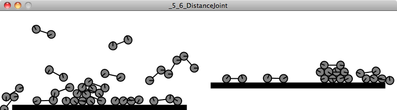
Exercise 5.6

Create a simulation of a bridge by using distance joints to connect a sequence of circles (or rectangles) as illustrated to the right. Assign a density of zero to lock the endpoints in place. Experiment with different values to make the bridge more or less “springy.” It should also be noted that the joints themselves have no physical geometry, so in order for your bridge not to have holes, spacing between the nodes will be important.

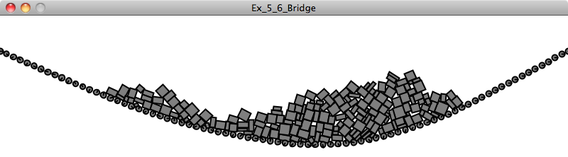
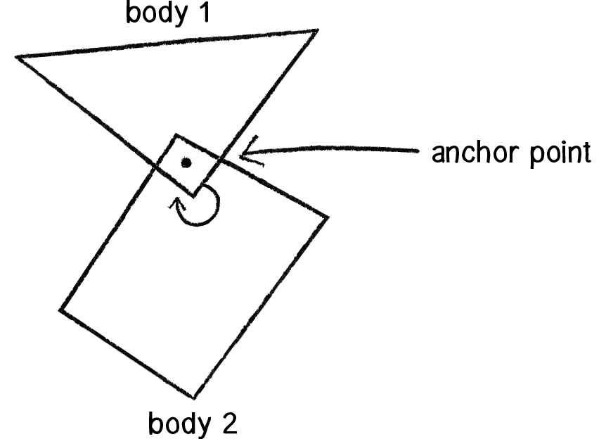
Figure 5.11

Another joint you can create in Box2D is a revolute joint. A revolute joint connects two Box2D bodies at a common anchor point, which can also be referred to as a “hinge.” The joint has an “angle” that describes the relative rotation of each body. To use a revolute joint, we follow the same steps we did with the distance joint.

Box box1 = new Box();
Box box2 = new Box();

RevoluteJointDef rjd = new RevoluteJointDef();

rjd.initialize(box1.body, box2.body, box1.body.getWorldCenter());

rjd.enableMotor = true;

rjd.motorSpeed = PI*2;

rjd.maxMotorTorque = 1000.0;

rjd.enableLimit = true;
rjd.lowerAngle = -PI/8;
rjd.upperAngle = PI/8;

Step 4: Create the joint.

Show Raw RevoluteJoint joint = (RevoluteJoint) box2d.world.createJoint(rjd);

RevoluteJoint joint = (RevoluteJoint) box2d.world.createJoint(rjd);

Let’s take a look at all of these steps together in a class called Windmill, which connects two boxes with a revolute joint. In this case, box1 has a density of zero, so only box2 spins around a fixed point.

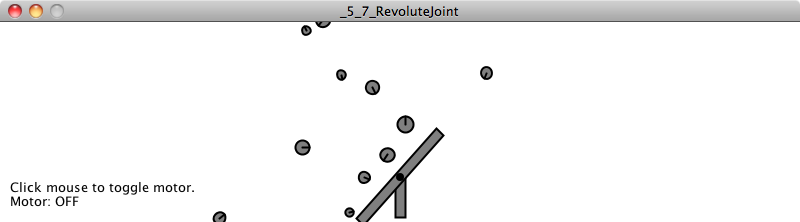
Example 5.7: Spinning Windmill

Show Raw class Windmill { // Our “Windmill” is two boxes and one joint. RevoluteJoint joint; Box box1; Box box2; Windmill(float x, float y) { //[full] In this example, the Box class expects a boolean argument that will be used to determine if the Box is fixed or not. See website for the Box class code. box1 = new Box(x,y,120,10,false); box2 = new Box(x,y,10,40,true); //[end] RevoluteJointDef rjd = new RevoluteJointDef(); //[offset-down] The joint connects two bodies and is anchored at the center of the first body. rjd.initialize(box1.body, box2.body, box1.body.getWorldCenter()); // A motor! rjd.motorSpeed = PI*2; rjd.maxMotorTorque = 1000.0; rjd.enableMotor = true; //[offset-down] Create the Joint. joint = (RevoluteJoint) box2d.world.createJoint(rjd); } //[full] Turning the motor on or off void toggleMotor() { boolean motorstatus = joint.isMotorEnabled(); joint.enableMotor(!motorstatus); } //[end] void display() { box1.display(); box2.display(); } }

class Windmill {
 

Our “Windmill” is two boxes and one joint.

  RevoluteJoint joint;
  Box box1;
  Box box2;
 
  Windmill(float x, float y) {
 

In this example, the Box class expects a boolean argument that will be used to determine if the Box is fixed or not. See website for the Box class code.

    box1 = new Box(x,y,120,10,false);
    box2 = new Box(x,y,10,40,true);
 
 

 
    RevoluteJointDef rjd = new RevoluteJointDef();

The joint connects two bodies and is anchored at the center of the first body.

    rjd.initialize(box1.body, box2.body, box1.body.getWorldCenter());
 
 
 

A motor!

    rjd.motorSpeed = PI*2;
    rjd.maxMotorTorque = 1000.0;
    rjd.enableMotor = true;
 

Create the Joint.

    joint = (RevoluteJoint) box2d.world.createJoint(rjd);
  }
 

Turning the motor on or off

  void toggleMotor() {
    boolean motorstatus = joint.isMotorEnabled();
    joint.enableMotor(!motorstatus);
  }

 
  void display() {
    box1.display();
    box2.display();
  }
}

Exercise 5.7

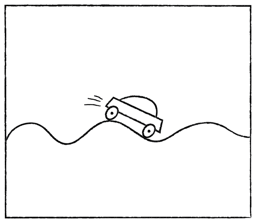
Use a revolute joint for the wheels of a car. Use motors so that the car drives autonomously. Try using a chain shape for the road’s surface.

The last joint we’ll look at is a mouse joint. A mouse joint is typically used for moving a body with the mouse. However, it can also be used to drag an object around the screen according to some arbitrary x and y. The joint functions by pulling the body towards a “target” position.

Before we look at the MouseJoint object itself, let’s ask ourselves why we even need it in the first place. If you look at the Box2D documentation, there is a function called setTransform() that specifically “sets the position of the body’s origin and rotation (radians).” If a body has a position, can’t we just assign the body’s position to the mouse?

Show Raw Vec2 mouse = box2d.screenToWorld(x,y); body.setTransform(mouse,0);

Vec2 mouse = box2d.screenToWorld(x,y);
body.setTransform(mouse,0);

While this will in fact move the body, it will also have the unfortunate result of breaking the physics. Let’s imagine you built a teleportation machine that allows you to teleport from your bedroom to your kitchen (good for late-night snacking). Now, go ahead and rewrite Newton’s laws of motion to account for the possibility of teleportation. Not so easy, right? Box2D has the same problem. If you manually assign the location of an body, it’s like saying “teleport that body” and Box2D no longer knows how to compute the physics properly. However, Box2D does allow you to tie a rope to yourself and get a friend of yours to stand in the kitchen and drag you there. This is what the MouseJoint does. It’s like a string you attach to a body and pull towards a target.

Let’s look at making this joint, assuming we have a Box object called box. This code will look identical to our distance joint with one small difference.

Show Raw // Just like before, define the Joint. MouseJointDef md = new MouseJointDef(); // Whoa, this is new! md.bodyA = box2d.getGroundBody(); //[bold] // Attach the Box body. md.bodyB = box.body; // Set properties. md.maxForce = 5000.0; md.frequencyHz = 5.0; md.dampingRatio = 0.9; // Create the joint. MouseJoint mouseJoint = (MouseJoint) box2d.world.createJoint(md);.

Just like before, define the Joint.

MouseJointDef md = new MouseJointDef();
 

Whoa, this is new!

md.bodyA = box2d.getGroundBody();

Attach the Box body.

md.bodyB = box.body;
 

Set properties.

md.maxForce = 5000.0;
md.frequencyHz = 5.0;
md.dampingRatio = 0.9;
 

Create the joint.

MouseJoint mouseJoint = (MouseJoint) box2d.world.createJoint(md);.

So, what’s this line of code all about?

Show Raw md.bodyA = box2d.getGroundBody(); //[bold]

md.bodyA = box2d.getGroundBody();

Well, as we’ve stated, a joint is a connection between two bodies. With a mouse joint, we’re saying that the second body is, well, the ground. Hmm. What the heck is the ground in Box2D? One way to imagine it is to think of the screen as the ground. What we’re doing is making a joint that connects a rectangle drawn on the window with the Processing window itself. And the point in the window to which the connection is tied is a moving target.

Once we have a mouse joint, we’ll want to update the target location continually while the sketch is running.

Show Raw Vec2 mouseWorld = box2d.coordPixelsToWorld(mouseX,mouseY); mouseJoint.setTarget(mouseWorld);

Vec2 mouseWorld = box2d.coordPixelsToWorld(mouseX,mouseY);
mouseJoint.setTarget(mouseWorld);

To make this work in an actual Processing sketch, we’ll want to have the following:

1. Box class—An object that references a Box2D body.

2. Spring class—An object that manages the mouse joint that drags the Box object around.

3. Main tab—Whenever mousePressed() is called, the mouse joint is created; whenever mouseReleased() is called, the mouse joint is destroyed. This allows us to interact with a body only when the mouse is pressed.

Let’s take a look at the main tab. You can find the rest of the code for the Box and Spring classes via the book website.

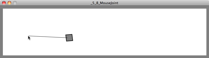
Example 5.8: MouseJoint demonstration

Show Raw PBox2D box2d; // One Box Box box; // Object to manage MouseJoint Spring spring; void setup() { size(400,300); box2d = new PBox2D(this); box2d.createWorld(); box = new Box(width/2,height/2); // The MouseJoint is really null until we click the mouse. spring = new Spring(); } void mousePressed() { // Was the mouse clicked inside the Box? if (box.contains(mouseX, mouseY)) { // If so, attach the MouseJoint. spring.bind(mouseX,mouseY,box); } } void mouseReleased() { // When the mouse is released, we’re done with the MouseJoint. spring.destroy(); } void draw() { background(255); box2d.step(); // We must always update the MouseJoint’s target. spring.update(mouseX,mouseY); box.display(); spring.display(); }

PBox2D box2d;
 

One Box

Box box;

Object to manage MouseJoint

Spring spring;
 
void setup() {
  size(400,300);
  box2d = new PBox2D(this);
  box2d.createWorld();
 
  box = new Box(width/2,height/2);

The MouseJoint is really null until we click the mouse.

  spring = new Spring();
}
 
void mousePressed() {

Was the mouse clicked inside the Box?

  if (box.contains(mouseX, mouseY)) {

If so, attach the MouseJoint.

    spring.bind(mouseX,mouseY,box);
  }
}
 
void mouseReleased() {

When the mouse is released, we’re done with the MouseJoint.

  spring.destroy();
}
 
void draw() {
  background(255);
 
  box2d.step();
 

We must always update the MouseJoint’s target.

  spring.update(mouseX,mouseY);
 
  box.display();
  spring.display();
}

Exercise 5.8

Use a mouse joint to move a Box2D body around the screen according to an algorithm or input other than the mouse. For example, assign it a location according to Perlin noise or key presses. Or build your own controller using an Arduino.

It’s worth noting that while the technique for dragging an object around using a MouseJoint is useful, Box2D also allows a body to have a KINEMATIC type.

Show Raw BodyDef bd = new BodyDef(); // Setting the body type to Kinematic bd.type = BodyType.KINEMATIC;

BodyDef bd = new BodyDef();

Setting the body type to Kinematic

bd.type = BodyType.KINEMATIC;

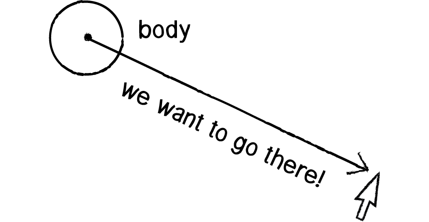
Figure 5.12

Kinematic bodies can be controlled by the user by setting their velocity directly. For example, let’s say you want an object to follow a target (like your mouse). You could create a vector that points from a body’s location to a target.

Show Raw Vec2 pos = body.getWorldCenter(); Vec2 target = box2d.coordPixelsToWorld(mouseX,mouseY); // A vector pointing from the body position to the Mouse Vec2 v = target.sub(pos);

Vec2 pos = body.getWorldCenter();
Vec2 target = box2d.coordPixelsToWorld(mouseX,mouseY);

A vector pointing from the body position to the Mouse

Vec2 v = target.sub(pos);

Once you have that vector, you could assign it to the body’s velocity so that it moves to the target.

Show Raw // Assigning a body’s velocity directly, overriding physics! body.setLinearVelocity(v);

Assigning a body’s velocity directly, overriding physics!

body.setLinearVelocity(v);

You can also do the same with angular velocity (or leave it alone and allow the physics to take over).

It is important to note that kinematic bodies do not collide with other kinematic or static bodies. In these cases, the mouse joint strategy is preferable.

Exercise 5.9

Redo Exercise 5.8, but use a kinematic body instead.

5.12 Bringing It All Back Home to Forces

In Chapter 2, we spent a lot of time thinking about building environments with multiple forces. An object might respond to gravitational attraction, wind, air resistance, etc. Clearly there are forces at work in Box2D as we watch rectangles and circles spin and fly around the screen. But so far, we’ve only had the ability to manipulate a single global force—gravity.

  box2d = new PBox2D(this);
  box2d.createWorld();

  box2d.setGravity(0, -20);

If we want to use any of our Chapter 2 techniques with Box2D, we need look no further than our trusty applyForce() function. In our Mover class we wrote a function called applyForce(), which received a vector, divided it by mass, and accumulated it into the mover’s acceleration. With Box2D, the same function exists, but we don’t need to write it ourselves. Instead, we can call the Box2D body’s applyForce() function!

class Box {
  Body body;
 
  void applyForce(Vec2 force) {
    Vec2 pos = body.getWorldCenter();

    body.applyForce(force, pos);
  }
}

Here we are receiving a force vector and passing it along to the Box2D Body object. The key difference is that Box2D is a more sophisticated engine than our examples from Chapter 2. Our earlier forces examples assumed that the force was always applied at the mover’s center. Here we get to specify exactly where on the body the force is applied. In the above code, we’re just applying it to the center by asking the body for its center, but this could be adjusted.

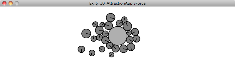
Let’s say we wanted to use a gravitational attraction force. Remember the code we wrote back in Chapter 2 in our Attractor class?

PVector attract(Mover m) {
  PVector force = PVector.sub(location,m.location);
  float distance = force.mag();
  distance = constrain(distance,5.0,25.0);
  force.normalize();
  float strength = (g * mass * m.mass) / (distance * distance);
  force.mult(strength);
  return force;
}

We can rewrite the exact same function using Vec2 instead and use it in a Box2D example. Note how for our force calculation we can stay completely within the Box2D coordinate system and never think about pixels.

Vec2 attract(Mover m) {

  Vec2 pos = body.getWorldCenter();
  Vec2 moverPos = m.body.getWorldCenter();
  Vec2 force = pos.sub(moverPos);
  float distance = force.length();
  distance = constrain(distance,1,5);
  force.normalize();
  float strength = (G * 1 * m.body.m_mass) / (distance * distance);

  force.mulLocal(strength);
  return force;
}

Exercise 5.10

Take any example you made previously using a force calculation and bring that force calculation into Box2D.

5.13 Collision Events

Now we’ve seen a survey of what can be done with Box2D. Since this book is not called “The Nature of Box2D,” it’s not my intention to cover every single possible feature of the Box2D engine. But hopefully by looking at the basics of building bodies, shapes, and joints, when it comes time to use an aspect of Box2D that we haven’t covered, the skills we’ve gained here will make that process considerably less painful. There is one more feature of Box2D, however, that I do think is worth covering.

Let’s ask a question you’ve likely been wondering about:

What if I want something to happen when two Box2D bodies collide? I mean, don’t get me wrong—I’m thrilled that Box2D is handling all of the collisions for me. But if it takes care of everything for me, how am I supposed to know when things are happening?

Your first thoughts when considering an event during which two objects collide might be as follows: Well, if I know all the bodies in the system, and I know where they are all located, then I can just start comparing the locations, see which ones are intersecting, and determine that they’ve collided. That’s a nice thought, but hello??!? The whole point of using Box2D is that Box2D will take care of that for us. If we are going to do the geometry to test for intersection ourselves, then all we’re doing is re-implementing Box2D.

Of course, Box2D has thought of this problem before. It’s a pretty common one. After all, if you intend to make a bajillion dollars selling some game called Angry Birds, you better well make something happen when an ill-tempered pigeon smashes into a cardboard box. Box2D alerts you to moments of collision with something called an “interface.” It’s worth learning about interfaces, an advanced feature of object-oriented programming. You can take a look at the Java Interface Tutorial as well as the JBox2D ContactListener class. (I have also included an example on the website that demonstrates using the interface directly.)

If you are using PBox2D, as we are here, you don’t need to implement your own interface. Detecting collision events is done through a callback function. Much like mousePressed() is triggered when the mouse is pressed, beginContact() is triggered when two shapes collide.

void mousePressed() {
  println("The mouse was pressed!");
}
 

void beginContact(Contact cp) {
  println("Something collided in the Box2D World!");
}

Before the above will work, you must first let PBox2D know you intend to listen for collisions. (This allows the library to reduce overhead by default; it won’t bother listening if it doesn’t have to.)

void setup() {
  box2d = new PBox2D(this);
  box2d.createWorld();

  box2d.listenForCollisions();
}

There are four collision event callbacks.

The details behind preSolve() and postSolve() are beyond the scope of this book; however, we are going to take a close look at beginContact(), which will cover the majority of conventional cases in which you want to trigger an action when a collision occurs. endContact() works identically to beginContact(), the only difference being that it occurs the moment bodies separate.

beginContact() is written as follows:

void beginContact(Contact cp) {
 
}

Notice that the function above includes an argument of type Contact. A Contact object includes all the data associated with a collision—the geometry and the forces. Let’s say we have a Processing sketch with Particle objects that store a reference to a Box2D body. Here is the process we are going to follow.

Fixture f1 = cp.getFixtureA();
Fixture f2 = cp.getFixtureB();

Body b1 = f1.getBody();
Body b2 = f2.getBody();

Step 3: Bodies, could you tell me which Particles you are associated with?

OK, this is the harder part. After all, Box2D doesn’t know anything about our code. Sure, it is doing all sorts of stuff to keep track of the relationships between shapes and bodies and joints, but it’s up to us to manage our own objects and their associations with Box2D elements. Luckily for us, Box2D provides a function that allows us to attach our Processing object (a Particle) to a Box2D body via the setUserData() and getUserData() methods.

Let’s take a look at the constructor in our Particle class where the body is made. We are expanding our body-making procedure by one line of code, noted below.

Show Raw class Particle { Body body; Particle(float x, float y, float r) { BodyDef bd = new BodyDef(); bd.position = box2d.coordPixelsToWorld(x, y); bd.type = BodyType.DYNAMIC; body = box2d.createBody(bd); CircleShape cs = new CircleShape(); cs.m_radius = box2d.scalarPixelsToWorld(r); body.createFixture(fd,1); // "this" refers to this Particle object. // We are telling the Box2D Body to store a // reference to this Particle that we can // access later. body.setUserData(this); //[bold] }

class Particle {
  Body body;
 
  Particle(float x, float y, float r) {
    BodyDef bd = new BodyDef();
    bd.position = box2d.coordPixelsToWorld(x, y);
    bd.type = BodyType.DYNAMIC;
    body = box2d.createBody(bd);
    CircleShape cs = new CircleShape();
    cs.m_radius = box2d.scalarPixelsToWorld(r);
    body.createFixture(fd,1);
 

"this" refers to this Particle object. We are telling the Box2D Body to store a reference to this Particle that we can access later.

    body.setUserData(this);
  }

Later, in our addContact() function, once we know the body, we can access the Particle object with getUserData().

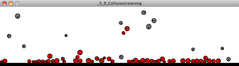
Example 5.9: CollisionListening

Show Raw void beginContact(Contact cp) { Fixture f1 = cp.getFixtureA(); Fixture f2 = cp.getFixtureB(); Body b1 = f1.getBody(); Body b2 = f2.getBody(); //[full] When we pull the “user data” object out of the Body object, we have to remind our program that it is a Particle object. Box2D doesn’t know this. Particle p1 = (Particle) b1.getUserData(); Particle p2 = (Particle) b2.getUserData(); //[end] //[full] Once we have the particles, we can do anything to them. Here we // just call a function that changes their color. p1.change(); p2.change(); //[end] }

void beginContact(Contact cp) {
 
  Fixture f1 = cp.getFixtureA();
  Fixture f2 = cp.getFixtureB();
 
  Body b1 = f1.getBody();
  Body b2 = f2.getBody();
 

When we pull the “user data” object out of the Body object, we have to remind our program that it is a Particle object. Box2D doesn’t know this.

  Particle p1 = (Particle) b1.getUserData();
  Particle p2 = (Particle) b2.getUserData();
 
 

Once we have the particles, we can do anything to them. Here we just call a function that changes their color.

  p1.change();
  p2.change();
 

}

Now, in many cases, we cannot assume that the objects that collided are all Particle objects. We might have a sketch with Boundary objects, Particle objects, Box objects, etc. So often we will have to query the “user data” and find out what kind of object it is before proceeding.

Show Raw // Getting a generic object Object o1 = b1.getUserData(); // Asking that object if it’s a Particle if (o1.getClass() == Particle.class) { Particle p = (Particle) o1; p.change(); }

Getting a generic object

  Object o1 = b1.getUserData();

Asking that object if it’s a Particle

  if (o1.getClass() == Particle.class) {
    Particle p = (Particle) o1;
    p.change();
  }

It should also be noted that due to how Box2D triggers these callbacks, you cannot create or destroy Box2D entities inside of beginContact(), endContact(), preSolve(), or postSolve(). If you want to do this, you’ll need to set a variable inside an object (something like: markForDeletion = true), which you check during draw() and then delete objects.

Exercise 5.11

Consider how polymorphism could help in the above case. Build an example in which several classes extend one class and therefore eliminate the need for such testing.

Exercise 5.12

Create a simulation in which Particle objects disappear when they collide with one another. Use the methodology I just described.

5.14 A Brief Interlude—Integration Methods

Has the following ever happened to you? You’re at a fancy cocktail party regaling your friends with tall tales of software physics simulations. Someone pipes up: “Enchanting! But what integration method are you using?” “What?!” you think to yourself. “Integration?”

Maybe you’ve heard the term before. Along with “differentiation,” it’s one of the two main operations in calculus. Right, calculus. The good news is, we’ve gotten through about 90% of the material in this book related to physics simulation and we haven’t really needed to dive into calculus. But as we’re coming close to finishing this topic, it’s worth taking a moment to examine the calculus behind what we have been doing and how it relates to the methodology in certain physics libraries (like Box2D and the upcoming toxiclibs).

Let’s begin by answering the question: “What does integration have to do with location, velocity, and acceleration?” Well, first let’s define differentiation, the process of finding a “derivative.” The derivative of a function is a measure of how a function changes over time. Consider location and its derivative. Location is a point in space, while velocity is change in location over time. Therefore, velocity can be described as the “derivative” of location. What is acceleration? The change in velocity over time—i.e. the “derivative” of velocity.

Now that we understand the derivative (differentiation), we can define the integral (integration) as the inverse of the derivative. In other words, the integral of an object’s velocity over time tells us the object’s new location when that time period ends. Location is the integral of velocity, and velocity is the integral of acceleration. Since our physics simulation is founded upon the process of calculating acceleration based on forces, we need integration to figure out where the object is after a certain period of time (like one frame of animation!)

So we’ve been doing integration all along! It looks like this:

velocity.add(acceleration);
location.add(velocity);

The above methodology is known as Euler integration (named for the mathematician Leonhard Euler, pronounced “Oiler”) or the Euler method. It’s essentially the simplest form of integration and very easy to implement in our code (see the two lines above!) However, it is not necessarily the most efficient form, nor is it close to being the most accurate. Why is Euler inaccurate? Let’s think about it this way. When you drive a car down the road pressing the gas pedal with your foot and accelerating, does the car sit in one location at time equals one second, then disappear and suddenly reappear in a new location at time equals two seconds, and do the same thing for three seconds, and four, and five? No, of course not. The car moves continuously down the road. But what’s happening in our Processing sketch? A circle is at one location at frame 0, another at frame 1, another at frame 2. Sure, at thirty frames per second, we’re seeing the illusion of motion. But we only calculate a new location every N units of time, whereas the real world is perfectly continuous. This results in some inaccuracies, as shown in the diagram below:

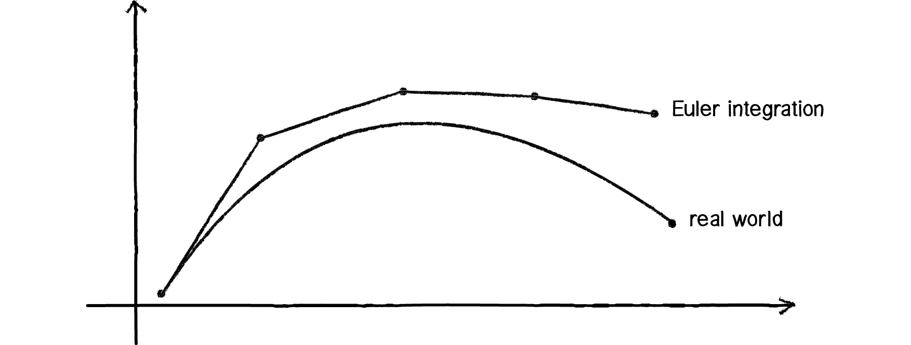
Figure 5.13

The “real world” is the curve; Euler simulation is the series of line segments.

One option to improve on Euler is to use smaller timesteps—instead of once per frame, we could recalculate an object’s location twenty times per frame. But this isn’t practical; our sketch would then run too slowly.

I still believe that Euler is the best method for learning the basics, and it’s also perfectly adequate for most of the projects we might make in Processing. Anything we lose in efficiency or inaccuracy we make up in ease of use and understandability. For better accuracy, Box2D uses something called symplectic Euler or semi-explicit Euler, a slight modification of Euler.

There is also an integration method called Runge-Kutta (named for German mathematicians C. Runge and M. W. Kutta), which is used in some physics engines.

A very popular integration method that our next physics library uses is known as “Verlet integration.” A simple way to describe Verlet integration is to think of our typical motion algorithm without velocity. After all, we don’t really need to store the velocity. If we always know where an object was at one point in time and where it is now, we can extrapolate its velocity. Verlet integration does precisely this, though instead of having a variable for velocity, it calculates velocity while the program is running. Verlet integration is particularly well suited for particle systems, especially particle systems with spring connections between the particles. We don’t need to worry about the details because toxiclibs, as we’ll see below, takes care of them for us. However, if you are interested, here is the seminal paper on Verlet physics, from which just about every Verlet computer graphics simulation is derived: "Advanced Character Physics". And of course, you can find out more about Verlet integration from Wikipedia.

5.15 Verlet Physics with toxiclibs

From toxiclibs.org:

“toxiclibs is an independent, open source library collection for computational design tasks with Java & Processing developed by Karsten “toxi” Schmidt (thus far). The classes are purposefully kept fairly generic in order to maximize re-use in different contexts ranging from generative design, animation, interaction/interface design, data visualization to architecture and digital fabrication, use as teaching tool and more.”

In other words, we should thank our lucky stars for toxiclibs. We are only going to focus on a few examples related to Verlet physics, but toxiclibs includes a suite of other wonderful packages that help with audio, color, geometry, and more. In particular, if you are looking to work with form and fabrication in Processing, take a look at the geometry package. Demos can be found at Open Processing.

We should note that toxiclibs was designed specifically for use with Processing. This is great news. The trouble we had with making Box2D work in Processing (multiple coordinate systems, Box2D vs. JBox2D vs. PBox2D) is not an issue here. toxiclibs is a library that you just download, stick in your libraries folder, and use. And the coordinate system that we’ll use for the physics engine is the coordinate system of Processing, so no translating back and forth. In addition, toxiclibs is not limited to a 2D world; all of the physics simulations and functions work in both two and three dimensions. So how do you decide which library you should use? Box2D or toxiclibs? If you fall into one of the following two categories, your decision is a bit easier:

1. My project involves collisions. I have circles, squares, and other strangely shaped objects that knock each other around and bounce off each other.

In this case, you are going to need Box2D. toxiclibs does not handle collisions.

2. My project involves lots of particles flying around the screen. Sometimes they attract each other. Sometimes they repel each other. And sometimes they are connected with springs.

In this case, toxiclibs is likely your best choice. It is simpler to use than Box2D and particularly well suited to connected systems of particles. toxiclibs is also very high performance, due to the speed of the Verlet integration algorithm (not to mention the fact that the program gets to ignore all of the collision geometry).

Here is a little chart that covers some of the features for each physics library.

PVector a = new PVector(1,-1);
PVector b = new PVector(3,4);
a.add(b);

Vec2D a = new Vec2D(1,-1);
Vec2D b = new Vec2D(3,4);
a.addSelf(b);

PVector a = new PVector(1,-1);
PVector b = new PVector(3,4);
PVector c = PVector.add(a,b);

Vec2D a = new Vec2D(1,-1);
Vec2D b = new Vec2D(3,4);
Vec2D c = a.add(b);

PVector a = new PVector(1,-1);
float m = a.mag();
a.normalize();

Vec2D a = new Vec2D(1,-1);
float m = a.magnitude();
a.normalize();

import toxi.physics2d.*;
import toxi.physics2d.behaviors.*;
import toxi.geom.*;

VerletPhysics2D physics;
 
void setup() {

  physics=new VerletPhysics2D();

  physics.setWorldBounds(new Rect(0,0,width,height));

  physics.addBehavior(new GravityBehavior(new Vec2D(0,0.5)));
}

void draw() {

  physics.update();
}

5.16 Particles and Springs in toxiclibs

In the Box2D examples, we saw how we can create our own class (called, say, Particle) and include a reference to a Box2D body.

class Particle {
  Body body;

This technique is somewhat redundant since Box2D itself keeps track of all of the bodies in its world. However, it allows us to manage which body is which (and therefore how each body is drawn) without having to rely on iterating through Box2D’s internal lists.

Let’s look at how we might take the same approach with the class VerletParticle2D in toxiclibs. We want to make our own Particle class so that we can draw our particles a certain way and include any custom properties. We’d probably write our code as follows:

class Particle {

  VerletParticle2D p;
 
  Particle(Vec2D pos) {

    p = new VerletParticle2D(pos);
  }
 
  void display() {
    fill(0,150);
    stroke(0);

    ellipse(p.x,p.y,16,16);
  }
}

Looking at the above, we should first be thrilled to notice that drawing the particle is as simple as grabbing the x and y and using them. No awkward conversions between coordinate systems here since toxiclibs is designed to think in pixels. Second, you might notice that this Particle class’s sole purpose is to store a reference to a VerletParticle2D object. This hints at something. Remember our discussion of inheritance back in Chapter 4: Particle Systems? What is a Particle object other than an “augmented” VerletParticle? Why bother making a Verlet particle inside a particle when we could simply extend VerletParticle?

class Particle extends VerletParticle2D {
 
  Particle(Vec2D loc) {

    super(loc);
  }
 

  void display() {
    fill(175);
    stroke(0);

    ellipse(x,y,16,16);
  }
}

Remember our multi-step process with the Box2D examples? We had to ask the body for its location, then convert that location to pixels, then use that location in a drawing function. Now, because we have inherited everything from the VerletParticle class, our only step is to draw the shape at x and y!

Incidentally, it’s interesting to note that the VerletParticle2D class is a subclass of Vec2D. So in addition to inheriting everything from VerletParticle2D, our Particle class actually has all of the Vec2D functions available as well.

We can now create particles anywhere within our sketch.

  Particle p1 = new Particle(new Vec2D(100,20));
  Particle p2 = new Particle(new Vec2D(100,180));

Just making a particle isn’t enough, however. We have to make sure we tell our physics world about them with the addParticle() function.

  physics.addParticle(p1);
  physics.addParticle(p2);

If you look at the toxiclibs documentation, you’ll see that the addParticle() expects a VerletParticle2D object.

addParticle(VerletParticle2D particle)

And how can we then pass into the function our own Particle object? Remember that other tenet of object-oriented programming—polymorphism? Here, because our Particle class extends VerletParticle2D, we can choose to treat our particle in two different ways—as a Particle or as a VerletParticle2D. This is an incredibly powerful feature of object-oriented programming. If we build our custom classes based on classes from toxiclibs, we can use our objects in conjunction with all of the functions toxiclibs has to offer.

In addition to the VerletParticle class, toxiclibs has a set of classes that allow you to connect particles with spring forces. There are three types of springs in toxiclibs:

The inheritance and polymorphism technique we employed in the previous section also proves to be useful when creating springs. A spring expects two particles when it is created. And again, because our Particle class extends VerletParticle, a VerletSpring object will accept our Particle objects passed into the constructor. Let’s take a look at some example code that assumes the existence of our two previous particles p1 and p2 and creates a connection between them with a given rest length and strength.

float len = 80;

float strength = 0.01;
VerletSpring2D spring=new VerletSpring2D(p1,p2,len,strength);

Just as with particles, in order for the connection to actually be part of the physics world, we need to explicitly add it.

physics.addSpring(spring);

5.17 Putting It All Together: A Simple Interactive Spring

One thing we saw with Box2D is that the physics simulation broke down when we overrode it and manually set the location of a body. With toxiclibs, we don’t have this problem. If we want to move the location of a particle, we can simply set its x and y location manually. However, before we do so, it’s generally a good idea to call the lock() function.

lock() is typically used to lock a particle in place and is identical to setting a Box2D body’s density to 0. However, here we are going to show how to lock a particle temporarily, move it, and then unlock it so that it continues to move according to the physics simulation. 
Let’s say you want to move a given particle whenever you click the mouse.

  if (mousePressed) {

    p2.lock();
    p2.x = mouseX;
    p2.y = mouseY;
    p2.unlock();

  }

And now we’re ready to put all of these elements together in a simple example that connects two particles with a spring. One particle is locked in place, and the other can be moved by dragging the mouse. Note that this example is virtually identical to Example 3.11.

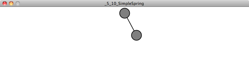
Example 5.10: Simple Spring with toxiclibs

import toxi.physics2d.*;
import toxi.physics2d.behaviors.*;
import toxi.geom.*;
 
VerletPhysics2D physics;
Particle p1;
Particle p2;
 
void setup() {
  size(640,360);
 

  physics=new VerletPhysics2D();
  physics.addBehavior(new GravityBehavior2D(new Vec2D(0,0.5)));
  physics.setWorldBounds(new Rect(0,0,width,height));
 

  p1 = new Particle(new Vec2D(100,20));
  p2 = new Particle(new Vec2D(100,180));

  p1.lock();
 

  VerletSpring2D spring=new VerletSpring2D(p1,p2,80,0.01);
 

  physics.addParticle(p1);
  physics.addParticle(p2);
  physics.addSpring(spring);
}
 
void draw() {

  physics.update();
 
  background(255);
 

  line(p1.x,p1.y,p2.x,p2.y);
  p1.display();
  p2.display();
 
  if (mousePressed) {

    p2.lock();
    p2.x = mouseX;
    p2.y = mouseY;
    p2.unlock();

  }
}
 

class Particle extends VerletParticle2D {
 
  Particle(Vec2D loc) {
    super(loc);
  }
 
  void display() {
    fill(175);
    stroke(0);
    ellipse(x,y,16,16);
  }
}

5.18 Connected Systems, Part I: String

The above example, two particles connected with a single spring, is the core building block for what toxiclibs’ physics is particularly well suited for: soft body simulations. For example, a string can be simulated by connecting a line of particles with springs. A blanket can be simulated by connecting a grid of particles with springs. And a cute, cuddly, squishy cartoon character can be simulated by a custom layout of particles connected with springs.

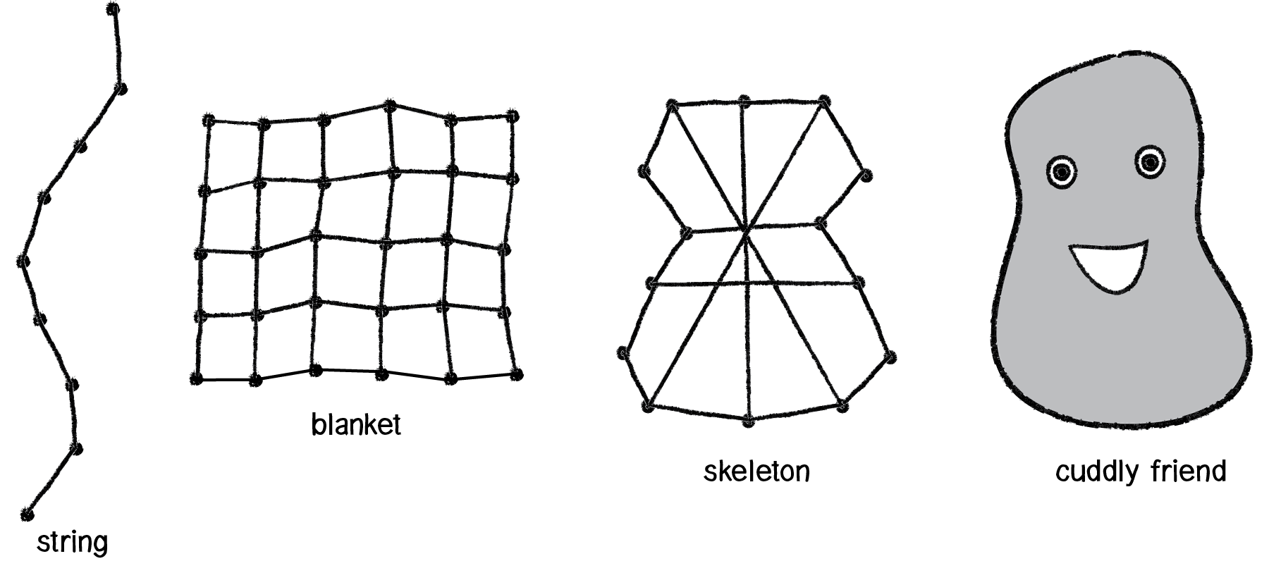
Figure 5.14

Let’s begin by simulating a “soft pendulum”—a bob hanging from a string, instead of a rigid arm like we had in Chapter 3. Let’s use the "string" in Figure 5.14 above as our model.

First, we’ll need a list of particles (let’s use the same Particle class we built in the previous example).

ArrayList<Particle> particles = new ArrayList<Particle>();

Now, let’s say we want to have 20 particles, all spaced 10 pixels apart.

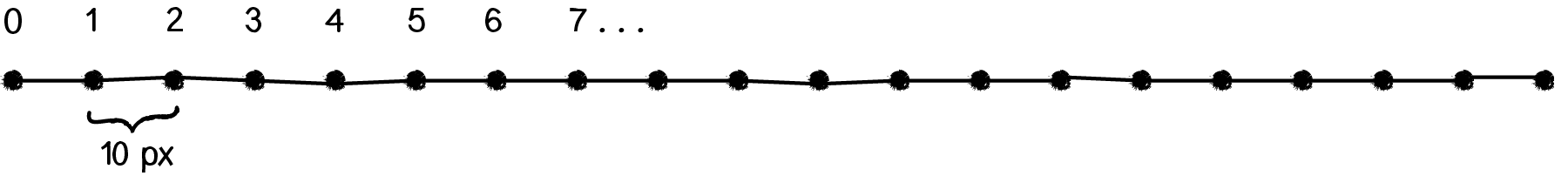
Figure 5.15

float len = 10;
float numParticles = 20;

We can loop from i equals 0 all the way up to 20, with each particle’s y location set to i * 10 so that the first particle is at (0,10), the second at (0,20), the third at (0,30), etc.

for(int i=0; i < numPoints; i++) {

  Particle particle=new Particle(i*len,10);

  physics.addParticle(particle);

  particles.add(particle);
}

Even though it’s a bit redundant, we’re going to add the particle to both the toxiclibs physics world and to our own list. In case we eventually have multiple strings, this will allow us to know which particles are connected to which strings.

Now for the fun part: It’s time to connect all the particles. Particle 1 will be connected to particle 0, particle 2 to particle 1, 3 to 2, 4 to 3, etc.

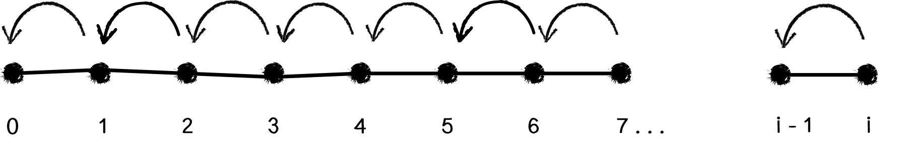
Figure 5.16

In other words, particle i needs to be connected to particle i-1 (except for when i equals zero).

if (i != 0) {

  Particle previous = particles.get(i-1);
 

  VerletSpring2D spring = new VerletSpring2D(particle,previous,len,strength);
 
 
 
 

  physics.addSpring(spring);
}

Now, what if we want the string to hang from a fixed point? We can lock one of the particles—the first, the last, the middle one, etc. Here’s how we would access the first particle (in the ArrayList) and lock it.

Particle head=particles.get(0);
head.lock();

And if we want to draw all the particles as being connected with a line, along with a circle for the last particle, we can use beginShape(), endShape(), and vertex(), accessing the particle locations from our ArrayList.

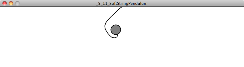
Example 5.11: Soft swinging pendulum

stroke(0);
noFill();
beginShape();
for (Particle p : particles) {

  vertex(p.x,p.y);
}
endShape();
Particle tail = particles.get(numPoints-1);

tail.display();

The full code available with the chapter download also demonstrates how to drag the tail particle with the mouse.

Exercise 5.13

Create a hanging cloth simulation using the technique above, but connect all the particles with a grid as demonstrated in the screenshot below.

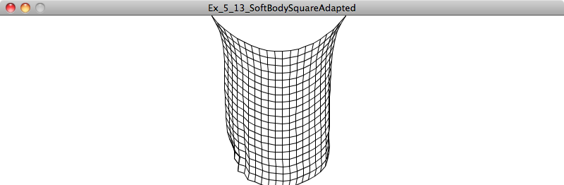
5.19 Connected Systems, Part II: Force-Directed Graph

Have you ever encountered the following scenario?

“I have a whole bunch of stuff I want to draw on the screen and I want all that stuff to be spaced out evenly in a nice, neat, organized manner. Otherwise I have trouble sleeping at night.”

This is not an uncommon problem in computational design. One solution is typically referred to as a “force-directed graph.” A force-directed graph is a visualization of elements—let’s call them “nodes”—in which the positions of those nodes are not manually assigned. Rather, the nodes arrange themselves according to a set of forces. While any forces can be used, a typical example involves spring forces. And so toxiclibs is perfect for this scenario.

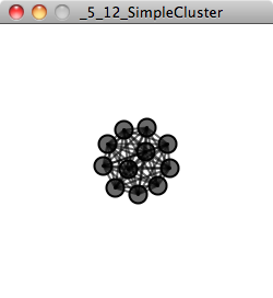
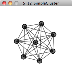
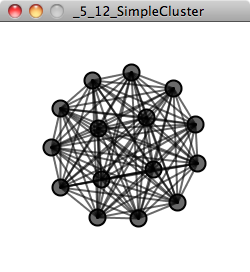
How do we implement the above?

First, we’ll need a Node class. This is the easy part; it can extend VerletParticle2D. Really, this is just what we did before, only we’re calling it Node now instead of Particle.

class Node extends VerletParticle2D {
  Node(Vec2D pos) {
    super(pos);
  }
 
  void display() {
    fill(0,150);
    stroke(0);
    ellipse(x,y,16,16);
  }
}

Next we can write a class called Cluster, which will describe a list of nodes.

class Cluster {
 
  ArrayList<Node> nodes;
 

  float diameter;
 
  Cluster(int n, float d, Vec2D center) {
    nodes = new ArrayList<Node>();
    diameter = d;
 
    for (int i = 0; i < n; i++) {

      nodes.add(new Node(center.add(Vec2D.randomVector())));
 
 
 
    }
  }

Let’s assume we added a display() function to draw all the nodes in the cluster and created a Cluster object in setup() and displayed it in draw(). If we ran the sketch as is, nothing would happen. Why? Because we forgot the whole force-directed graph part! We need to connect every single node to every other node with a force. But what exactly do we mean by that? Let’s assume we have four Node objects: 0, 1, 2 and 3. Here are our connections:

0 connected to 1
0 connected to 2
0 connected to 3
1 connected to 2
1 connected to 3
2 connected to 3

Notice two important details about our connection list.

So how do we write code to make these connections for N number of nodes?

Look at the left column. It reads: 000 11 22. So we know we need to access each node in the list from 0 to N-1.

    for (int i = 0; i < nodes.size()-1; i++) {
      VerletParticle2D ni = nodes.get(i);

Now, we know we need to connect node 0 to nodes 1,2,3. For node 1: 2,3. For node 2: 3. So for every node i, we must loop from i+1 until the end of the list.

      for (int j = i+1; j < nodes.size(); j++) {
        VerletParticle2D nj = nodes.get(j);

With every two Nodes we find, all we have to do then is make a spring.

        physics.addSpring(new VerletSpring2D(ni,nj,diameter,0.01));
      }
    }

Assuming those connections are made in the Cluster constructor, we can now create a cluster in our main tab and see the results!

Example 5.12: Cluster

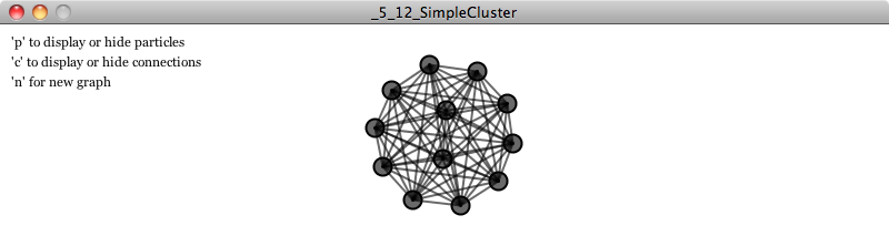
import toxi.geom.*;
import toxi.physics2d.*;
 
VerletPhysics2D physics;
Cluster cluster;
 
void setup() {
  size(300,300);
  physics=new VerletPhysics2D();

  cluster = new Cluster(8,100,new Vec2D(width/2,height/2));
}
 
void draw() {
  physics.update();
  background(255);

  cluster.display();
}

Exercise 5.15

Expand the force-directed graph to have more than one Cluster object. Use a VerletMinDistanceSpring2D object to connect cluster to cluster.

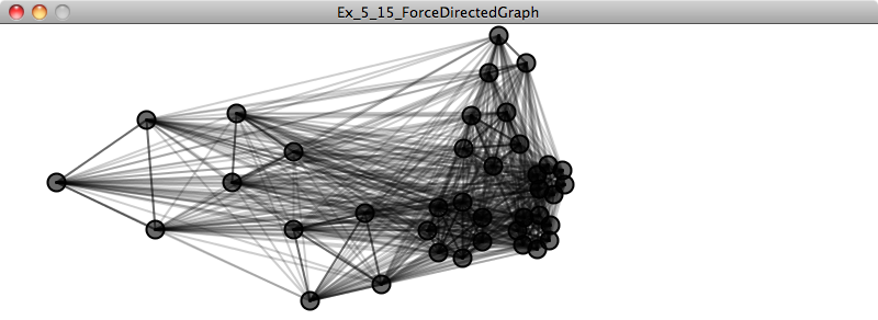
5.20 Attraction and Repulsion Behaviors

When we looked at adding an attraction force to Box2D, we found that the Box2D Body class included an applyForce() function. All we needed to do was calculate the attraction force (Force = G * mass1 * mass2 / distance squared) as a vector and apply it to the body. toxiclibs VerletParticle class also includes a function called addForce() that we can use to apply any calculated force to a particle.

However, toxiclibs also takes this idea one step further by allowing us to attach some common forces (let’s call them “behaviors”) to particles, calculating them and applying them for us! For example, if we attach an AttractionBehavior object to a particle, then all other particles in the physics world will be attracted to that particle.

Let’s say we have a Particle class (that extends VerletParticle).

Particle p = new Particle(new Vec2D(200,200));

Once we’ve made a Particle object, we can create an AttractionBehavior object associated with that particle.

float distance = 20;
float strength = 0.1;
AttractionBehavior behavior = new AttractionBehavior(p, distance, strength);

Notice how the behavior is created with two parameters—distance and strength. The distance specifies the range within which the behavior will be applied. For example, in the above scenario, only other particles within twenty pixels will feel the attraction force. The strength, of course, specifies how strong the force is.

Finally, in order for the force to be activated, the behavior needs to be added to the physics world.

physics.addBehavior(behavior);

This means everything that lives in the physics simulation will always be attracted to that particle, as long as it is within the distance threshold.

Even though toxiclibs does not handle collisions, you can create a collision-like effect by adding a repulsive behavior to each and every particle (so that every particle repels every other particle). Let’s look at how we might modify our Particle class to do this.

class Particle extends VerletParticle2D {
 

  float r;
 
  Particle (Vec2D loc) {
    super(loc);
    r = 4;

    physics.addBehavior(new AttractionBehavior(this, r*4, -1));
  }
 
  void display () {
    fill (255);
    stroke (255);
    ellipse (x, y, r*2, r*2);
  }
}

We could now recreate our attraction example by having a single Attractor object that exerts an attraction behavior over the entire window.

Example 5.13: Attraction/Repulsion

class Attractor extends VerletParticle2D {
 
  float r;
 
  Attractor (Vec2D loc) {
    super (loc);
    r = 24;