Chapter 2. Forces
“Don’t underestimate the Force.” — Darth Vader
In the final example of Chapter 1, we saw how we could calculate a dynamic acceleration based on a vector pointing from a circle on the screen to the mouse location. The resulting motion resembled a magnetic attraction between circle and mouse, as if some force were pulling the circle in towards the mouse. In this chapter we will formalize our understanding of the concept of a force and its relationship to acceleration. Our goal, by the end of this chapter, is to understand how to make multiple objects move around the screen and respond to a variety of environmental forces.
2.1 Forces and Newton’s Laws of Motion
Before we begin examining the practical realities of simulating forces in code, let’s take a conceptual look at what it means to be a force in the real world. Just like the word “vector,” “force” is often used to mean a variety of things. It can indicate a powerful intensity, as in “She pushed the boulder with great force” or “He spoke forcefully.” The definition of force that we care about is much more formal and comes from Isaac Newton’s laws of motion:
A force is a vector that causes an object with mass to accelerate.
The good news here is that we recognize the first part of the definition: a force is a vector. Thank goodness we just spent a whole chapter learning what a vector is and how to program with PVectors!
Let’s look at Newton’s three laws of motion in relation to the concept of a force.
Newton’s First Law
Newton’s first law is commonly stated as:
An object at rest stays at rest and an object in motion stays in motion.
However, this is missing an important element related to forces. We could expand it by stating:
An object at rest stays at rest and an object in motion stays in motion at a constant speed and direction unless acted upon by an unbalanced force.
By the time Newton came along, the prevailing theory of motion—formulated by Aristotle—was nearly two thousand years old. It stated that if an object is moving, some sort of force is required to keep it moving. Unless that moving thing is being pushed or pulled, it will simply slow down or stop. Right?
This, of course, is not true. In the absence of any forces, no force is required to keep an object moving. An object (such as a ball) tossed in the earth’s atmosphere slows down because of air resistance (a force). An object’s velocity will only remain constant in the absence of any forces or if the forces that act on it cancel each other out, i.e. the net force adds up to zero. This is often referred to as equilibrium. The falling ball will reach a terminal velocity (that stays constant) once the force of air resistance equals the force of gravity.

Figure 2.1: The pendulum doesn't move because all the forces cancel each other out (add up to a net force of zero).
In our Processing world, we could restate Newton’s first law as follows:
An object’s PVector velocity will remain constant if it is in a state of equilibrium.
Skipping Newton’s second law (arguably the most important law for our purposes) for a moment, let’s move on to the third law.
Newton’s Third Law
This law is often stated as:
For every action there is an equal and opposite reaction.
This law frequently causes some confusion in the way that it is stated. For one, it sounds like one force causes another. Yes, if you push someone, that someone may actively decide to push you back. But this is not the action and reaction we are talking about with Newton’s third law.
Let’s say you push against a wall. The wall doesn’t actively decide to push back on you. There is no “origin” force. Your push simply includes both forces, referred to as an “action/reaction pair.”
A better way of stating the law might be:
Forces always occur in pairs. The two forces are of equal strength, but in opposite directions.
Now, this still causes confusion because it sounds like these forces would always cancel each other out. This is not the case. Remember, the forces act on different objects. And just because the two forces are equal, it doesn’t mean that the movements are equal (or that the objects will stop moving).
Try pushing on a stationary truck. Although the truck is far more powerful than you, unlike a moving one, a stationary truck will never overpower you and send you flying backwards. The force you exert on it is equal and opposite to the force exerted on your hands. The outcome depends on a variety of other factors. If the truck is a small truck on an icy downhill, you’ll probably be able to get it to move. On the other hand, if it’s a very large truck on a dirt road and you push hard enough (maybe even take a running start), you could injure your hand.
And if you are wearing roller skates when you push on that truck?
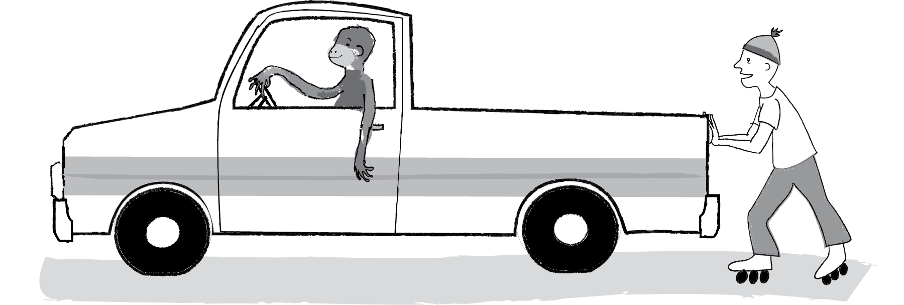
Figure 2.2
You’ll accelerate away from the truck, sliding along the road while the truck stays put. Why do you slide but not the truck? For one, the truck has a much larger mass (which we’ll get into with Newton’s second law). There are other forces at work too, namely the friction of the truck’s tires and your roller skates against the road.
Newton’s Third Law (as seen through the eyes of Processing)
If we calculate a PVector f that is a force of object A on object B, we must also apply the force—PVector.mult(f,-1);—that B exerts on object A.
We’ll see that in the world of Processing programming, we don’t always have to stay true to the above. Sometimes, such as in the case of see gravitational attraction between bodies, we’ll want to model equal and opposite forces. Other times, such as when we’re simply saying, “Hey, there’s some wind in the environment,” we’re not going to bother to model the force that a body exerts back on the air. In fact, we’re not modeling the air at all! Remember, we are simply taking inspiration from the physics of the natural world, not simulating everything with perfect precision.
2.2 Forces and Processing—Newton’s Second Law as a Function
And here we are at the most important law for the Processing programmer.
Newton’s Second Law
This law is stated as:
Force equals mass times acceleration.
Or:
Why is this the most important law for us? Well, let’s write it a different way.
Acceleration is directly proportional to force and inversely proportional to mass. This means that if you get pushed, the harder you are pushed, the faster you’ll move (accelerate). The bigger you are, the slower you’ll move.
Weight vs. Mass
The mass of an object is a measure of the amount of matter in the object (measured in kilograms).
Weight, though often mistaken for mass, is technically the force of gravity on an object. From Newton’s second law, we can calculate it as mass times the acceleration of gravity (w = m * g). Weight is measured in newtons.
Density is defined as the amount of mass per unit of volume (grams per cubic centimeter, for example).
Note that an object that has a mass of one kilogram on earth would have a mass of one kilogram on the moon. However, it would weigh only one-sixth as much.
Now, in the world of Processing, what is mass anyway? Aren’t we dealing with pixels? To start in a simpler place, let’s say that in our pretend pixel world, all of our objects have a mass equal to 1. F/ 1 = F. And so:
The acceleration of an object is equal to force. This is great news. After all, we saw in Chapter 1 that acceleration was the key to controlling the movement of our objects on screen. Location is adjusted by velocity, and velocity by acceleration. Acceleration was where it all began. Now we learn that force is truly where it all begins.
Let’s take our Mover class, with location, velocity, and acceleration.
Now our goal is to be able to add forces to this object, perhaps saying:
mover.applyForce(wind);or:
mover.applyForce(gravity);where wind and gravity are PVectors. According to Newton’s second law, we could implement this function as follows.
void applyForce(PVector force) { acceleration = force;
}
2.3 Force Accumulation
This looks pretty good. After all, acceleration = force is a literal translation of Newton’s second law (without mass). Nevertheless, there’s a pretty big problem here. Let’s return to what we are trying to accomplish: creating a moving object on the screen that responds to wind and gravity.
mover.applyForce(wind);
mover.applyForce(gravity);
mover.update();
mover.display();
Ok, let’s be the computer for a moment. First, we call applyForce() with wind. And so the Mover object’s acceleration is now assigned the PVector wind. Second, we call applyForce() with gravity. Now the Mover object’s acceleration is set to the gravity PVector. Third, we call update(). What happens in update()? Acceleration is added to velocity.
velocity.add(acceleration);We’re not going to see any error in Processing, but zoinks! We’ve got a major problem. What is the value of acceleration when it is added to velocity? It is equal to the gravity force. Wind has been left out! If we call applyForce() more than once, it overrides each previous call. How are we going to handle more than one force?
The truth of the matter here is that we started with a simplified statement of Newton’s second law. Here’s a more accurate way to put it:
Net Force equals mass times acceleration.
Or, acceleration is equal to the sum of all forces divided by mass. This makes perfect sense. After all, as we saw in Newton’s first law, if all the forces add up to zero, an object experiences an equilibrium state (i.e. no acceleration). Our implementation of this is through a process known as force accumulation. It’s actually very simple; all we need to do is add all of the forces together. At any given moment, there might be 1, 2, 6, 12, or 303 forces. As long as our object knows how to accumulate them, it doesn’t matter how many forces act on it.
void applyForce(PVector force) { acceleration.add(force);
}
Now, we’re not finished just yet. Force accumulation has one more piece. Since we’re adding all the forces together at any given moment, we have to make sure that we clear acceleration (i.e. set it to zero) before each time update() is called. Let’s think about wind for a moment. Sometimes the wind is very strong, sometimes it’s weak, and sometimes there’s no wind at all. At any given moment, there might be a huge gust of wind, say, when the user holds down the mouse.
if (mousePressed) {
PVector wind = new PVector(0.5,0);
mover.applyForce(wind);
}
When the user releases the mouse, the wind will stop, and according to Newton’s first law, the object will continue to move at a constant velocity. However, if we had forgotten to reset acceleration to zero, the gust of wind would still be in effect. Even worse, it would add onto itself from the previous frame, since we are accumulating forces! Acceleration, in our simulation, has no memory; it is simply calculated based on the environmental forces present at a moment in time. This is different than, say, location, which must remember where the object was in the previous frame in order to move properly to the next.
The easiest way to implement clearing the acceleration for each frame is to multiply the PVector by 0 at the end of update().
void update() {
velocity.add(acceleration);
location.add(velocity);
acceleration.mult(0);
}
2.4 Dealing with Mass
OK. We’ve got one tiny little addition to make before we are done with integrating forces into our Mover class and are ready to look at examples. After all, Newton’s second law is really , not . Incorporating mass is as easy as adding an instance variable to our class, but we need to spend a little more time here because a slight complication will emerge.
First we just need to add mass.
class Mover {
PVector location;
PVector velocity;
PVector acceleration;
float mass;Units of Measurement
Now that we are introducing mass, it’s important to make a quick note about units of measurement. In the real world, things are measured in specific units. We say that two objects are 3 meters apart, the baseball is moving at a rate of 90 miles per hour, or this bowling ball has a mass of 6 kilograms. As we’ll see later in this book, sometimes we will want to take real-world units into consideration. However, in this chapter, we’re going to ignore them for the most part. Our units of measurement are in pixels (“These two circles are 100 pixels apart”) and frames of animation (“This circle is moving at a rate of 2 pixels per frame”). In the case of mass, there isn’t any unit of measurement for us to use. We’re just going to make something up. In this example, we’re arbitrarily picking the number 10. There is no unit of measurement, though you might enjoy inventing a unit of your own, like “1 moog” or “1 yurkle.” It should also be noted that, for demonstration purposes, we’ll tie mass to pixels (drawing, say, a circle with a radius of 10). This will allow us to visualize the mass of an object. In the real world, however, size does not definitely indicate mass. A small metal ball could have a much higher mass than a large balloon due to its higher density.
Mass is a scalar (float), not a vector, as it’s just one number describing the amount of matter in an object. We could be fancy about things and compute the area of a shape as its mass, but it’s simpler to begin by saying, “Hey, the mass of this object is…um, I dunno…how about 10?”
Mover() {
location = new PVector(random(width),random(height));
velocity = new PVector(0,0);
acceleration = new PVector(0,0);
mass = 10.0;
}
This isn’t so great since things only become interesting once we have objects with varying mass, but it’ll get us started. Where does mass come in? We use it while applying Newton’s second law to our object.
void applyForce(PVector force) { force.div(mass);
    acceleration.add(force);
}Yet again, even though our code looks quite reasonable, we have a fairly major problem here. Consider the following scenario with two Mover objects, both being blown away by a wind force.
Mover m1 = new Mover();
Mover m2 = new Mover();
PVector wind = new PVector(1,0);
m1.applyForce(wind);
m2.applyForce(wind);
Again, let’s be the computer. Object m1 receives the wind force—(1,0)—divides it by mass (10), and adds it to acceleration.
m1 equals wind force: (1,0)
Divided by mass of 10: (0.1,0)
OK. Moving on to object m2. It also receives the wind force—(1,0). Wait. Hold on a second. What is the value of the wind force? Taking a closer look, the wind force is actually now—(0.1,0)!! Do you remember this little tidbit about working with objects? When you pass an object (in this case a PVector) into a function, you are passing a reference to that object. It’s not a copy! So if a function makes a change to that object (which, in this case, it does by dividing by mass) then that object is permanently changed! But we don’t want m2 to receive a force divided by the mass of object m1. We want it to receive that force in its original state—(1,0). And so we must protect ourselves and make a copy of the PVector f before dividing it by mass. Fortunately, the PVector class has a convenient method for making a copy—get(). get() returns a new PVector object with the same data. And so we can revise applyForce() as follows:
void applyForce(PVector force) { PVector f = force.get();
f.div(mass);
acceleration.add(f);
}
There’s another way we could write the above function, using the static method div(). For help with this exercise, review static methods in Chapter 1.
Exercise 2.2
Rewrite the applyForce() method using the static method div() instead of get().
void applyForce(PVector force) {
PVector f = _______.___(_____,____);
acceleration.add(f);
}
2.5 Creating Forces
Let’s take a moment to remind ourselves where we are. We know what a force is (a vector), and we know how to apply a force to an object (divide it by mass and add it to the object’s acceleration vector). What are we missing? Well, we have yet to figure out how we get a force in the first place. Where do forces come from?
In this chapter, we’ll look at two methods for creating forces in our Processing world.
Make up a force! After all, you are the programmer, the creator of your world. There’s no reason why you can’t just make up a force and apply it.
Model a force! Yes, forces exist in the real world. And physics textbooks often contain formulas for these forces. We can take these formulas, translate them into source code, and model real-world forces in Processing.
The easiest way to make up a force is to just pick a number. Let’s start with the idea of simulating wind. How about a wind force that points to the right and is fairly weak? Assuming a Mover object m, our code would look like:
PVector wind = new PVector(0.01,0);
m.applyForce(wind);
The result isn’t terribly interesting, but it is a good place to start. We create a PVector object, initialize it, and pass it into an object (which in turn will apply it to its own acceleration). If we wanted to have two forces, perhaps wind and gravity (a bit stronger, pointing down), we might write the following:
PVector wind = new PVector(0.01,0);
PVector gravity = new PVector(0,0.1);
m.applyForce(wind);
m.applyForce(gravity);
Now we have two forces, pointing in different directions with different magnitudes, both applied to object m. We’re beginning to get somewhere. We’ve now built a world for our objects in Processing, an environment to which they can actually respond.
Let’s look at how we could make this example a bit more exciting with many objects of varying mass. To do this, we’ll need a quick review of object-oriented programming. Again, we’re not covering all the basics of programming here (for that you can check out any of the intro Processing books listed in the introduction). However, since the idea of creating a world filled with objects is pretty fundamental to all the examples in this book, it’s worth taking a moment to walk through the steps of going from one object to many.
This is where we are with the Mover class as a whole. Notice how it is identical to the Mover class created in Chapter 1, with two additions—mass and a new applyForce() function.
class Mover {
PVector location;
PVector velocity;
PVector acceleration;
float mass;
Mover() {
mass = 1;
location = new PVector(30,30);
velocity = new PVector(0,0);
acceleration = new PVector(0,0);
}
void applyForce(PVector force) { PVector f = PVector.div(force,mass);
acceleration.add(f);
}
 void update() {
    velocity.add(acceleration);
    location.add(velocity);
    acceleration.mult(0);
 }
void display() {
stroke(0);
fill(175);
    ellipse(location.x,location.y,mass*16,mass*16);
  }
  void checkEdges() {
    if (location.x > width) {
      location.x = width;
      velocity.x *= -1;
    } else if (location.x < 0) {
      velocity.x *= -1;
      location.x = 0;
    }

    if (location.y > height) {
      velocity.y *= -1;
      location.y = height;
    }
  }
}
Now that our class is set, we can choose to create, say, one hundred Mover objects with an array.
Mover[] movers = new Mover[100];And then we can initialize all of those Mover objects in setup() with a loop.
void setup() {
  for (int i = 0; i < movers.length; i++) {
    movers[i] = new Mover();
  }
}
But now we have a small issue. If we refer back to the Mover object’s constructor…
Mover() { mass = 1;
location = new PVector(30,30);
    velocity = new PVector(0,0);
    acceleration = new PVector(0,0);
  }
…we discover that every Mover object is made exactly the same way. What we want are Mover objects of varying mass that start at varying locations. Here is where we need to increase the sophistication of our constructor by adding arguments.
Mover(float m, float x , float y) { mass = m;
location = new PVector(x,y);
    velocity = new PVector(0,0);
    acceleration = new PVector(0,0);
  }
Notice how the mass and location are no longer set to hardcoded numbers, but rather initialized via arguments passed through the constructor. This means we can create a variety of Mover objects: big ones, small ones, ones that start on the left side of the screen, ones that start on the right, etc.
Mover m1 = new Mover(10,0,height/2);Mover m1 = new Mover(0.1,width,height/2);With an array, however, we want to initialize all of the objects with a loop.
void setup() {
  for (int i = 0; i < movers.length; i++) {
    movers[i] = new Mover(random(0.1,5),0,0);
  }
}
For each mover created, the mass is set to a random value between 0.1 and 5, the starting x-location is set to 0, and the starting y-location is set to 0. Certainly, there are all sorts of ways we might choose to initialize the objects; this is just a demonstration of one possibility.
Once the array of objects is declared, created, and initialized, the rest of the code is simple. We run through every object, hand them each the forces in the environment, and enjoy the show.
Example 2.2: Forces acting on many objects
void draw() {
  background(255);

  PVector wind = new PVector(0.01,0);
PVector gravity = new PVector(0,0.1);
  for (int i = 0; i < movers.length; i++) {
    movers[i].applyForce(wind);
    movers[i].applyForce(gravity);
    movers[i].update();
    movers[i].display();
    movers[i].checkEdges();
  }
}
Note how in the above image, the smaller circles reach the right of the window faster than the larger ones. This is because of our formula: acceleration = force divided by mass. The larger the mass, the smaller the acceleration.
2.6 Gravity on Earth and Modeling a Force
You may have noticed something woefully inaccurate about this last example. The smaller the circle, the faster it falls. There is a logic to this; after all, we just stated (according to Newton’s second law) that the smaller the mass, the higher the acceleration. But this is not what happens in the real world. If you were to climb to the top of the Leaning Tower of Pisa and drop two balls of different masses, which one will hit the ground first? According to legend, Galileo performed this exact test in 1589, discovering that they fell with the same acceleration, hitting the ground at the same time. Why is this? As we will see later in this chapter, the force of gravity is calculated relative to an object’s mass. The bigger the object, the stronger the force. So if the force is scaled according to mass, it is canceled out when acceleration is divided by mass. We can implement this in our sketch rather easily by multiplying our made-up gravity force by mass.
Example 2.3: Gravity scaled by mass
for (int i = 0; i < movers.length; i++) {

    PVector wind = new PVector(0.001,0);
    float m = movers[i].mass;
    PVector gravity = new PVector(0,0.1*m);
    movers[i].applyForce(wind);
    movers[i].applyForce(gravity);

    movers[i].update();
    movers[i].display();
    movers[i].checkEdges();
  }
While the objects now fall at the same rate, because the strength of the wind force is independent of mass, the smaller objects still accelerate to the right more quickly.
Making up forces will actually get us quite far. The world of Processing is a pretend world of pixels and you are its master. So whatever you deem appropriate to be a force, well by golly, that’s the force it should be. Nevertheless, there may come a time where you find yourself wondering: “But how does it really all work?”
Open up any high school physics textbook and you will find some diagrams and formulas describing many different forces—gravity, electromagnetism, friction, tension, elasticity, and more. In this chapter we’re going to look at two forces—friction and gravity. The point we’re making here is not that friction and gravity are fundamental forces that you always need to have in your Processing sketches. Rather, we want to evaluate these two forces as case studies for the following process:
Understanding the concept behind a force
Deconstructing the force’s formula into two parts:
How do we compute the force’s direction?
How do we compute the force’s magnitude?
Translating that formula into Processing code that calculates a PVector to be sent through our Mover's applyForce() function
If we can follow the above steps with two forces, then hopefully if you ever find yourself Googling “atomic nuclei weak nuclear force” at 3 a.m., you will have the skills to take what you find and adapt it for Processing.
Dealing with formulae
OK, in a moment we’re going to write out the formula for friction. This isn’t the first time we’ve seen a formula in this book; we just finished up our discussion of Newton’s second law, (or force = mass * acceleration). We didn’t spend a lot of time worrying about this formula because it’s a nice and simple one. Nevertheless, it’s a scary world out there. Just take a look at the equation for a “normal” distribution, which we covered (without looking at the formula) in the Introduction.
What we’re seeing here is that formulas like to use a lot of symbols (quite often letters from the Greek alphabet). Let’s take a look at the formula for friction.
If it’s been a while since you’ve looked at a formula from a math or physics textbook, there are three key points that are important to cover before we move on.
Evaluate the right side, assign to the left side. This is just like in code! What we’re doing here is evaluating the right side of the equation and assigning it to the left. In the case above, we want to calculate the force of friction—the left side tells us what we want to calculate and the right side tells us how to do it.
Are we talking about a vector or a scalar? It’s important for us to realize that in some cases, we’ll be looking at a vector; in others, a scalar. For example, in this case the force of friction is a vector. We can see that by the arrow above the word “friction.” It has a magnitude and direction. The right side of the equation also has a vector, as indicated by the symbol , which in this case stands for the velocity unit vector.
When symbols are placed next to each other, we mean for them to be multiplied. The formula above actually has four elements: -1, μ, N, and . We want to multiply them together and read the formula as:
2.7 Friction
Let’s begin with friction and follow our steps.
Friction is a dissipative force. A dissipative force is one in which the total energy of a system decreases when an object is in motion. Let’s say you are driving a car. When you press your foot down on the brake pedal, the car’s brakes use friction to slow down the motion of the tires. Kinetic energy (motion) is converted into thermal energy (heat). Whenever two surfaces come into contact, they experience friction. A complete model of friction would include separate cases for static friction (a body at rest against a surface) and kinetic friction (a body in motion against a surface), but for our purposes, we are only going to look at the kinetic case.
Here’s the formula for friction:
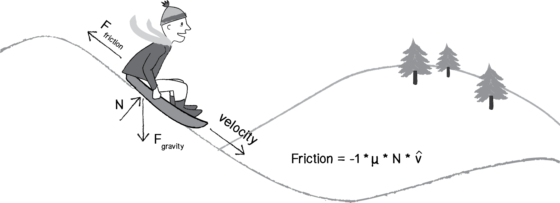
Figure 2.3
It’s now up to us to separate this formula into two components that determine the direction of friction as well as the magnitude. Based on the diagram above, we can see that friction points in the opposite direction of velocity. In fact, that’s the part of the formula that says -1 * , or -1 times the velocity unit vector. In Processing, this would mean taking the velocity vector, normalizing it, and multiplying by -1.
PVector friction = velocity.get();
friction.normalize();
friction.mult(-1);Notice two additional steps here. First, it’s important to make a copy of the velocity vector, as we don’t want to reverse the object’s direction by accident. Second, we normalize the vector. This is because the magnitude of friction is not associated with how fast it is moving, and we want to start with a friction vector of magnitude 1 so that it can easily be scaled.
According to the formula, the magnitude is μ * N. μ, the Greek letter mu (pronounced “mew”), is used here to describe the coefficient of friction. The coefficient of friction establishes the strength of a friction force for a particular surface. The higher it is, the stronger the friction; the lower, the weaker. A block of ice, for example, will have a much lower coefficient of friction than, say, sandpaper. Since we’re in a pretend Processing world, we can arbitrarily set the coefficient based on how much friction we want to simulate.
float c = 0.01;Now for the second part: N. N refers to the normal force, the force perpendicular to the object’s motion along a surface. Think of a vehicle driving along a road. The vehicle pushes down against the road with gravity, and Newton’s third law tells us that the road in turn pushes back against the vehicle. That’s the normal force. The greater the gravitational force, the greater the normal force. As we’ll see in the next section, gravity is associated with mass, and so a lightweight sports car would experience less friction than a massive tractor trailer truck. With the diagram above, however, where the object is moving along a surface at an angle, computing the normal force is a bit more complicated because it doesn’t point in the same direction as gravity. We’ll need to know something about angles and trigonometry.
All of these specifics are important; however, in Processing, a “good enough” simulation can be achieved without them. We can, for example, make friction work with the assumption that the normal force will always have a magnitude of 1. When we get into trigonometry in the next chapter, we’ll remember to return to this question and make our friction example a bit more sophisticated. Therefore:
float normal = 1;Now that we have both the magnitude and direction for friction, we can put it all together…
float c = 0.01;
float normal = 1;
float frictionMag = c*normal;

PVector friction = velocity.get();
friction.mult(-1);
friction.normalize();
friction.mult(frictionMag);…and add it to our “forces” example, where many objects experience wind, gravity, and now friction:
No friction
With friction
Example 2.4: Including friction
void draw() {
  background(255);

  PVector wind = new PVector(0.001,0);
  PVector gravity = new PVector(0,0.1);

  for (int i = 0; i < movers.length; i++) {

    float c = 0.01;
    PVector friction = movers[i].velocity.get();
    friction.mult(-1);
    friction.normalize();
    friction.mult(c);
    movers[i].applyForce(friction);
    movers[i].applyForce(wind);
    movers[i].applyForce(gravity);

    movers[i].update();
    movers[i].display();
    movers[i].checkEdges();
  }

}
Running this example, you’ll notice that the circles don’t even make it to the right side of the window. Since friction continuously pushes against the object in the opposite direction of its movement, the object continuously slows down. This can be a useful technique or a problem depending on the goals of your visualization.
Exercise 2.4
Create pockets of friction in a Processing sketch so that objects only experience friction when crossing over those pockets. What if you vary the strength (friction coefficient) of each area? What if you make some pockets feature the opposite of friction—i.e., when you enter a given pocket you actually speed up instead of slowing down?
2.8 Air and Fluid Resistance
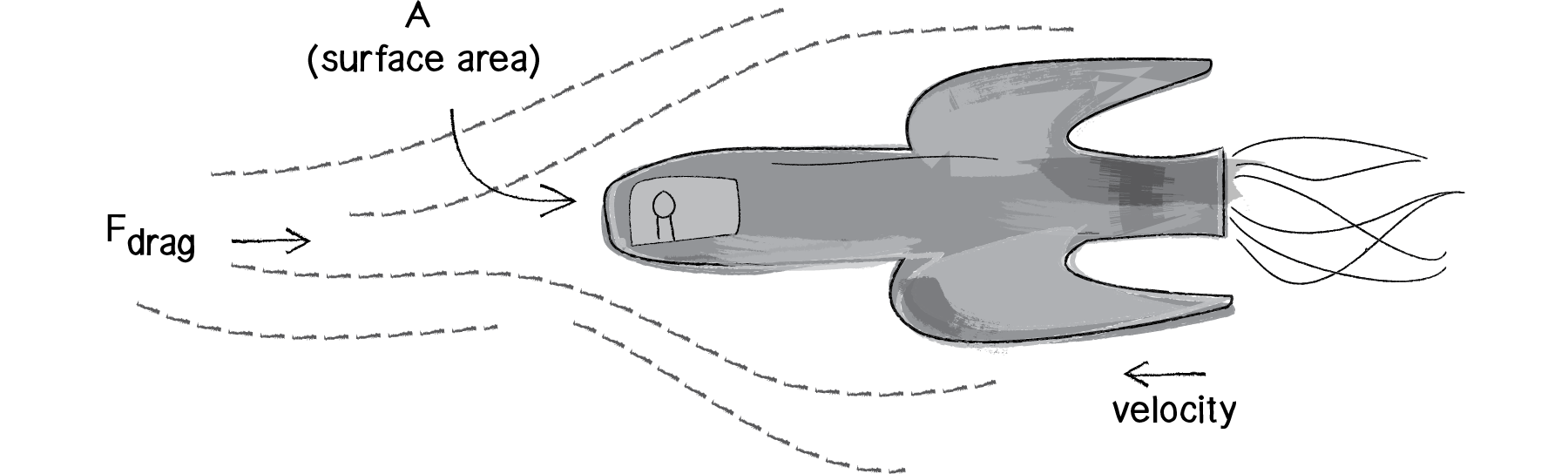
Figure 2.4
Friction also occurs when a body passes through a liquid or gas. This force has many different names, all really meaning the same thing: viscous force, drag force, fluid resistance. While the result is ultimately the same as our previous friction examples (the object slows down), the way in which we calculate a drag force will be slightly different. Let’s look at the formula:
Now let’s break this down and see what we really need for an effective simulation in Processing, making ourselves a much simpler formula in the process.
refers to drag force, the vector we ultimately want to compute and pass into our applyForce() function.
- 1/2 is a constant: -0.5. This is fairly irrelevant in terms of our Processing world, as we will be making up values for other constants anyway. However, the fact that it is negative is important, as it tells us that the force is in the opposite direction of velocity (just as with friction).
is the Greek letter rho, and refers to the density of the liquid, something we don’t need to worry about. We can simplify the problem and consider this to have a constant value of 1.
refers to the speed of the object moving. OK, we’ve got this one! The object’s speed is the magnitude of the velocity vector: velocity.magnitude(). And just means squared or * .
refers to the frontal area of the object that is pushing through the liquid (or gas). An aerodynamic Lamborghini, for example, will experience less air resistance than a boxy Volvo. Nevertheless, for a basic simulation, we can consider our object to be spherical and ignore this element.
is the coefficient of drag, exactly the same as the coefficient of friction (). This is a constant we’ll determine based on whether we want the drag force to be strong or weak.
Look familiar? It should. This refers to the velocity unit vector, i.e. velocity.normalize(). Just like with friction, drag is a force that points in the opposite direction of velocity.
Now that we’ve analyzed each of these components and determined what we need for a simple simulation, we can reduce our formula to:

Figure 2.5: Our simplified drag force formula
or:
float c = 0.1;
float speed = v.mag();
float dragMagnitude = c * speed * speed;
PVector drag = velocity.get();
drag.mult(-1);
drag.normalize();
drag.mult(dragMagnitude);Let’s implement this force in our Mover class example with one addition. When we wrote our friction example, the force of friction was always present. Whenever an object was moving, friction would slow it down. Here, let’s introduce an element to the environment—a “liquid” that the Mover objects pass through. The Liquid object will be a rectangle and will know about its location, width, height, and “coefficient of drag”—i.e., is it easy for objects to move through it (like air) or difficult (like molasses)? In addition, it should include a function to draw itself on the screen (and two more functions, which we’ll see in a moment).
class Liquid { float x,y,w,h;
float c;
Liquid(float x_, float y_, float w_, float h_, float c_) {
x = x_;
y = y_;
w = w_;
h = h_;
c = c_;
}
void display() {
noStroke();
fill(175);
rect(x,y,w,h);
}
}
The main program will now include a Liquid object reference as well as a line of code that initializes that object.
Liquid liquid;

void setup() {
  liquid = new Liquid(0, height/2, width, height/2, 0.1);
}
Now comes an interesting question: how do we get the Mover object to talk to the Liquid object? In other words, we want to execute the following:
When a mover passes through a liquid it experiences a drag force.
…or in object-oriented speak (assuming we are looping through an array of Mover objects with index i):
if (movers[i].isInside(liquid)) { movers[i].drag(liquid);
}
The above code tells us that we need to add two functions to the Mover class: (1) a function that determines if a Mover object is inside the Liquid object, and (2) a function that computes and applies a drag force on the Mover object.
The first is easy; we can simply use a conditional statement to determine if the location vector rests inside the rectangle defined by the liquid.
boolean isInside(Liquid l) { if (location.x>l.x && location.x<l.x+l.w && location.y>l.y && location.y<l.y+l.h)
{
return true;
} else {
return false;
}
}
The drag() function is a bit more complicated; however, we’ve written the code for it already. This is simply an implementation of our formula. The drag force is equal to the coefficient of drag multiplied by the speed of the Mover squared in the opposite direction of velocity!
void drag(Liquid l) {
float speed = velocity.mag();
float dragMagnitude = l.c * speed * speed;
PVector drag = velocity.get();
drag.mult(-1);
drag.normalize();
drag.mult(dragMagnitude);
applyForce(drag);
}
And with these two functions added to the Mover class, we’re ready to put it all together in the main tab:
Mover[] movers = new Mover[100];
Liquid liquid;
void setup() {
size(360, 640);
for (int i = 0; i < movers.length; i++) {
movers[i] = new Mover(random(0.1,5),0,0);
}
liquid = new Liquid(0, height/2, width, height/2, 0.1);
}
void draw() {
background(255);
liquid.display();
for (int i = 0; i < movers.length; i++) {
if (movers[i].isInside(liquid)) {
  movers[i].drag(liquid);
}
float m = 0.1*movers[i].mass;
    PVector gravity = new PVector(0, m);
    movers[i].applyForce(gravity);

    movers[i].update();
    movers[i].display();
    movers[i].checkEdges();
  }
}
Running the example, you should notice that we are simulating balls falling into water. The objects only slow down when crossing through the gray area at the bottom of the window (representing the liquid). You’ll also notice that the smaller objects slow down a great deal more than the larger objects. Remember Newton’s second law? A = F / M. Acceleration equals force divided by mass. A massive object will accelerate less. A smaller object will accelerate more. In this case, the acceleration we’re talking about is the “slowing down” due to drag. The smaller objects will slow down at a greater rate than the larger ones.
Exercise 2.5
Take a look at our formula for drag again: drag force = coefficient * speed * speed. The faster an object moves, the greater the drag force against it. In fact, an object not moving in water experiences no drag at all. Expand the example to drop the balls from different heights. How does this affect the drag as they hit the water?
2.9 Gravitational Attraction
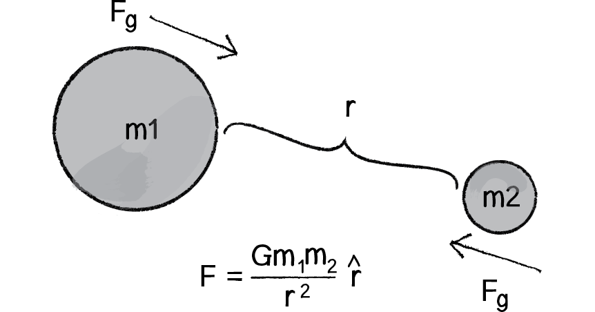
Figure 2.6
Probably the most famous force of all is gravity. We humans on earth think of gravity as an apple hitting Isaac Newton on the head. Gravity means that stuff falls down. But this is only our experience of gravity. In truth, just as the earth pulls the apple towards it due to a gravitational force, the apple pulls the earth as well. The thing is, the earth is just so freaking big that it overwhelms all the other gravity interactions. Every object with mass exerts a gravitational force on every other object. And there is a formula for calculating the strengths of these forces, as depicted in Figure 2.6.
Let’s examine this formula a bit more closely.
F refers to the gravitational force, the vector we ultimately want to compute and pass into our applyForce() function.
G is the universal gravitational constant, which in our world equals 6.67428 x 10⁻¹¹ meters cubed per kilogram per second squared. This is a pretty important number if your name is Isaac Newton or Albert Einstein. It’s not an important number if you are a Processing programmer. Again, it’s a constant that we can use to make the forces in our world weaker or stronger. Just making it equal to one and ignoring it isn’t such a terrible choice either.
m1 and m2 are the masses of objects 1 and 2. As we saw with Newton’s second law (), mass is also something we could choose to ignore. After all, shapes drawn on the screen don’t actually have a physical mass. However, if we keep these values, we can create more interesting simulations in which “bigger” objects exert a stronger gravitational force than smaller ones.
refers to the unit vector pointing from object 1 to object 2. As we’ll see in a moment, we can compute this direction vector by subtracting the location of one object from the other.
r2 refers to the distance between the two objects squared. Let’s take a moment to think about this a bit more. With everything on the top of the formula—G, m1, m2—the bigger its value, the stronger the force. Big mass, big force. Big G, big force. Now, when we divide by something, we have the opposite. The strength of the force is inversely proportional to the distance squared. The farther away an object is, the weaker the force; the closer, the stronger.
Hopefully by now the formula makes some sense to us. We’ve looked at a diagram and dissected the individual components of the formula. Now it’s time to figure out how we translate the math into Processing code. Let’s make the following assumptions.
We have two objects, and:
Each object has a location: PVector location1 and PVector location2.
Each object has a mass: float mass1 and float mass2.
There is a variable float G for the universal gravitational constant.
Given these assumptions, we want to compute PVector force, the force of gravity. We’ll do it in two parts. First, we’ll compute the direction of the force in the formula above. Second, we’ll calculate the strength of the force according to the masses and distance.
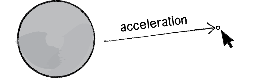
Figure 2.7
Remember in Chapter 1, when we figured out how to have an object accelerate towards the mouse? (See Figure 2.7.)
A vector is the difference between two points. To make a vector that points from the circle to the mouse, we simply subtract one point from another:
PVector dir = PVector.sub(mouse,location);In our case, the direction of the attraction force that object 1 exerts on object 2 is equal to:
PVector dir = PVector.sub(location1,location2);
dir.normalize();
Don’t forget that since we want a unit vector, a vector that tells us about direction only, we’ll need to normalize the vector after subtracting the locations.
OK, we’ve got the direction of the force. Now we just need to compute the magnitude and scale the vector accordingly.
float m = (G * mass1 * mass2) / (distance * distance);
dir.mult(m);
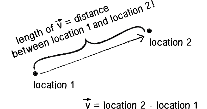
Figure 2.8
The only problem is that we don’t know the distance. G, mass1, and mass2 were all givens, but we’ll need to actually compute distance before the above code will work. Didn’t we just make a vector that points all the way from one location to another? Wouldn’t the length of that vector be the distance between two objects?
Well, if we add just one line of code and grab the magnitude of that vector before normalizing it, then we’ll have the distance.
PVector force = PVector.sub(location1,location2);
float distance = force.magnitude();
float m = (G * mass1 * mass2) / (distance * distance);
force.normalize();
force.mult(m);
Note that I also renamed the PVector “dir” as “force.” After all, when we’re finished with the calculations, the PVector we started with ends up being the actual force vector we wanted all along.
Now that we’ve worked out the math and the code for calculating an attractive force (emulating gravity), we need to turn our attention to applying this technique in the context of an actual Processing sketch. In Example 2.1, you may recall how we created a simple Mover object—a class with PVector’s location, velocity, and acceleration as well as an applyForce(). Let’s take this exact class and put it in a sketch with:
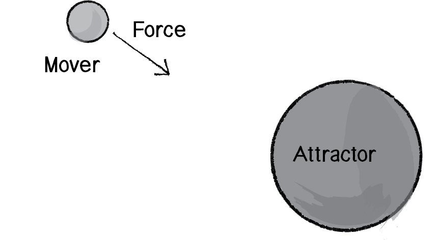
Figure 2.9
A single Mover object.
A single Attractor object (a new class that will have a fixed location).
The Mover object will experience a gravitational pull towards the Attractor object, as illustrated in Figure 2.9.
We can start by making the new Attractor class very simple—giving it a location and a mass, along with a function to display itself (tying mass to size).
class Attractor { float mass;
PVector location;
Attractor() {
location = new PVector(width/2,height/2);
mass = 20;
}
void display() {
stroke(0);
fill(175,200);
ellipse(location.x,location.y,mass*2,mass*2);
}
}
And in our main program, we can add an instance of the Attractor class.
Mover m;
Attractor a;

void setup() {
  size(640,360);
  m = new Mover();
  a = new Attractor();
}

void draw() {
  background(255);
  a.display();

  m.update();
  m.display();
}
This is a good structure: a main program with a Mover and an Attractor object, and a class to handle the variables and behaviors of movers and attractors. The last piece of the puzzle is how to get one object to attract the other. How do we get these two objects to talk to each other?
There are a number of ways we could do this. Here are just a few possibilities.
| Task | Function |
|---|---|
| 1. A function that receives both an Attractor and a Mover: | attraction(a,m); |
| 2. A function in the Attractor class that receives a Mover: | a.attract(m); |
| 3. A function in the Mover class that receives an Attractor: | m.attractedTo(a); |
| 4. A function in the Attractor class that receives a Mover and returns a PVector, which is the attraction force. That attraction force is then passed into the Mover's applyForce() function: |
PVector f = a.attract(m); m.applyForce(f); |
and so on. . .
It’s good to look at a range of options for making objects talk to each other, and you could probably make arguments for each of the above possibilities. I’d like to at least discard the first one, since an object-oriented approach is really a much better choice over an arbitrary function not tied to either the Mover or Attractor class. Whether you pick option 2 or option 3 is the difference between saying “The attractor attracts the mover” or “The mover is attracted to the attractor.” Number 4 is really my favorite, at least in terms of where we are in this book. After all, we spent a lot of time working out the applyForce() function, and I think our examples will be clearer if we continue with the same methodology.
In other words, where we once had:
PVector f = new PVector(0.1,0);
m.applyForce(f);
We now have:
PVector f = a.attract(m);
m.applyForce(f);
And so our draw() function can now be written as:
void draw() {
  background(255);
  PVector f = a.attract(m);
  m.applyForce(f);
  m.update();

  a.display();
  m.display();

}
We’re almost there. Since we decided to put the attract() function inside of the Attractor class, we’ll need to actually write that function. The function needs to receive a Mover object and return a PVector, i.e.:
PVector attract(Mover m) {

}
And what goes inside that function? All of that nice math we worked out for gravitational attraction!
PVector attract(Mover m) {
  PVector force = PVector.sub(location,m.location);
  float distance = force.mag();
  force.normalize();
  float strength = (G * mass * m.mass) / (distance * distance);
  force.mult(strength);
  return force;
}
And we’re done. Sort of. Almost. There’s one small kink we need to work out. Let’s look at the above code again. See that symbol for divide, the slash? Whenever we have one of these, we need to ask ourselves the question: What would happen if the distance happened to be a really, really small number or (even worse!) zero??! Well, we know we can’t divide a number by 0, and if we were to divide a number by something like 0.0001, that is the equivalent of multiplying that number by 10,000! Yes, this is the real-world formula for the strength of gravity, but we don’t live in the real world. We live in the Processing world. And in the Processing world, the mover could end up being very, very close to the attractor and the force could become so strong the mover would just fly way off the screen. And so with this formula, it’s good for us to be practical and constrain the range of what distance can actually be. Maybe, no matter where the Mover actually is, we should never consider it less than 5 pixels or more than 25 pixels away from the attractor.
distance = constrain(distance,5,25);For the same reason that we need to constrain the minimum distance, it’s useful for us to do the same with the maximum. After all, if the mover were to be, say, 500 pixels from the attractor (not unreasonable), we’d be dividing the force by 250,000. That force might end up being so weak that it’s almost as if we’re not applying it at all.
Now, it’s really up to you to decide what behaviors you want. But in the case of, “I want reasonable-looking attraction that is never absurdly weak or strong,” then constraining the distance is a good technique.
Our Mover class hasn’t changed at all, so let’s just look at the main program and the Attractor class as a whole, adding a variable G for the universal gravitational constant. (On the website, you’ll find that this example also has code that allows you to move the Attractor object with the mouse.)
Mover m;
Attractor a;

void setup() {
  size(640,360);
  m = new Mover();
  a = new Attractor();
}

void draw() {
  background(255);
  PVector force = a.attract(m);
  m.applyForce(force);
  m.update();

  a.display();
  m.display();
}

class Attractor {
  float mass;
  PVector location;
  float G;

  Attractor() {
    location = new PVector(width/2,height/2);
    mass = 20;
    G = 0.4;
  }

  PVector attract(Mover m) {
    PVector force = PVector.sub(location,m.location);
    float distance = force.mag();
    distance = constrain(distance,5.0,25.0);


    force.normalize();
    float strength = (G * mass * m.mass) / (distance * distance);
    force.mult(strength);
    return force;
  }

  void display() {
    stroke(0);
    fill(175,200);
    ellipse(location.x,location.y,mass*2,mass*2);
  }
}
And we could, of course, expand this example using an array to include many Mover objects, just as we did with friction and drag:
Example 2.7: Attraction with many Movers
Mover[] movers = new Mover[10];

Attractor a;

void setup() {
  size(400,400);
  for (int i = 0; i < movers.length; i++) {
    movers[i] = new Mover(random(0.1,2),random(width),random(height));
  }
  a = new Attractor();
}

void draw() {
  background(255);

  a.display();

  for (int i = 0; i < movers.length; i++) {
    PVector force = a.attract(movers[i]);
    movers[i].applyForce(force);

    movers[i].update();
    movers[i].display();
  }

}
Exercise 2.8
In the example above, we have a system (i.e. array) of Mover objects and one Attractor object. Build an example that has systems of both movers and attractors. What if you make the attractors invisible? Can you create a pattern/design from the trails of objects moving around attractors? See the Metropop Denim project by Clayton Cubitt and Tom Carden for an example.
Exercise 2.9
It’s worth noting that gravitational attraction is a model we can follow to develop our own forces. This chapter isn’t suggesting that you should exclusively create sketches that use gravitational attraction. Rather, you should be thinking creatively about how to design your own rules to drive the behavior of objects. For example, what happens if you design a force that is weaker the closer it gets and stronger the farther it gets? Or what if you design your attractor to attract faraway objects, but repel close ones?
2.10 Everything Attracts (or Repels) Everything
Hopefully, you found it helpful that we started with a simple scenario—one object attracts another object—and moved on to one object attracts many objects. However, it’s likely that you are going to find yourself in a slightly more complex situation: many objects attract each other. In other words, every object in a given system attracts every other object in that system (except for itself).
We’ve really done almost all of the work for this already. Let’s consider a Processing sketch with an array of Mover objects:
Mover[] movers = new Mover[10];

void setup() {
  size(400,400);
  for (int i = 0; i < movers.length; i++) {
    movers[i] = new Mover(random(0.1,2),random(width),random(height));
  }
}

void draw() {
  background(255);
  for (int i = 0; i < movers.length; i++) {
    movers[i].update();
    movers[i].display();
  }
}
The draw() function is where we need to work some magic. Currently, we’re saying: “for every mover i, update and display yourself.” Now what we need to say is: “for every mover i, be attracted to every other mover j, and update and display yourself.”
To do this, we need to nest a second loop.
for (int i = 0; i < movers.length; i++) { for (int j = 0; j < movers.length; j++) {
PVector force = movers[j].attract(movers[i]);
movers[i].applyForce(force);
}
movers[i].update();
movers[i].display();
}
In the previous example, we had an Attractor object with a function named attract(). Now, since we have movers attracting movers, all we need to do is copy the attract() function into the Mover class.
class Mover {

  // All the other stuff we had before plus. . .
  PVector attract(Mover m) {

    PVector force = PVector.sub(location,m.location);
    float distance = force.mag();
    distance = constrain(distance,5.0,25.0);
    force.normalize();

    float strength = (G * mass * m.mass) / (distance * distance);
    force.mult(strength);
    return force;
  }
}
Of course, there’s one small problem. When we are looking at every mover i and every mover j, are we OK with the times that i equals j? For example, should mover #3 attract mover #3? The answer, of course, is no. If there are five objects, we only want mover #3 to attract 0, 1, 2, and 4, skipping itself. And so, we finish this example by adding a simple conditional statement to skip applying the force when i equals j.
Example 2.8: Mutual attraction
Mover[] movers = new Mover[20];

float g = 0.4;

void setup() {
  size(400,400);
  for (int i = 0; i < movers.length; i++) {
    movers[i] = new Mover(random(0.1,2),random(width),random(height));
  }
}

void draw() {
  background(255);

  for (int i = 0; i < movers.length; i++) {
    for (int j = 0; j < movers.length; j++) {
      if (i != j) {
        PVector force = movers[j].attract(movers[i]);
        movers[i].applyForce(force);
      }
    }
    movers[i].update();
    movers[i].display();
  }
}
Exercise 2.10
Change the attraction force in Example 2.8 to a repulsion force. Can you create an example in which all of the Mover objects are attracted to the mouse, but repel each other? Think about how you need to balance the relative strength of the forces and how to most effectively use distance in your force calculations.
The Ecosystem Project
Step 2 Exercise:
Incorporate the concept of forces into your ecosystem. Try introducing other elements into the environment (food, a predator) for the creature to interact with. Does the creature experience attraction or repulsion to things in its world? Can you think more abstractly and design forces based on the creature’s desires or goals?

